YOLOv11
An Overview of the Key Architectural Enhancements — C3k2, SPPF, C2PSA and Multi-Task Heads
Rahima Khanam, Muhammad Hussain
Read the Paper on arXivPaper Overview
YOLOv11 (Khanam & Hussain, University of Huddersfield, October 2024) is a different kind of paper from most breakdowns on this site. YOLO11 itself was not introduced in a paper at all — Ultralytics (Jocher & Qiu) unveiled it at the YOLO Vision 2024 conference and shipped it as code. This arXiv report is the first written architectural analysis of that release: it reads the model apart, names its new modules, and places it in the nine-year YOLO lineage.
The analysis centres on three components. C3k2, a cheaper Cross Stage Partial block, replaces YOLOv8's C2f in the backbone, neck and head. SPPF (Spatial Pyramid Pooling — Fast) is retained at the end of the backbone. And C2PSA, a Cross Stage Partial block with spatial self-attention, is new — placed directly after SPPF, it is the attention mechanism YOLOv8 never had.
Around that sits the familiar backbone → neck → head layout, and an expanded task list: one architecture family serves object detection, instance segmentation, image classification, pose estimation, oriented bounding boxes (OBB) and tracking, each in nano, small, medium, large and extra-large sizes.
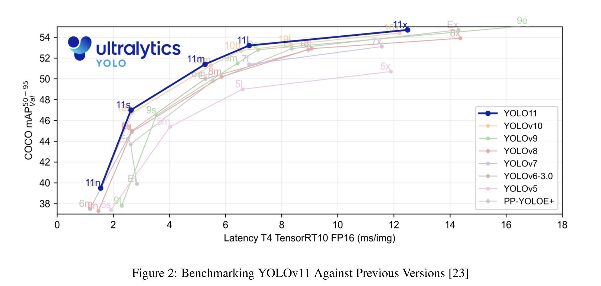
The headline numbers come from Ultralytics' published benchmark, which the paper reproduces as its Figure 2: YOLO11m reaches higher COCO mAP than YOLOv8m with 22% fewer parameters, and YOLO11x reaches roughly 54.5% mAP at about 13 ms on a T4 GPU — the top of the latency/accuracy frontier among YOLO versions. Read it as a guided tour of a production detector rather than a new method: the value is in seeing why each block is shaped the way it is.
Chapter Roadmap
Click any topic to jump in
Nine Years of YOLO
From the 2015 single-stage detector to YOLOv10's NMS-free training — the lineage YOLO11 inherits from.
Backbone, Neck, Head
YOLO11 keeps YOLOv8's three-part layout and swaps in three new modules: C3k2, SPPF + C2PSA.
Three new building blocks
C3k2 Block
A cheaper Cross Stage Partial block that replaces C2f everywhere — with a c3k switch for deeper inner modules.
SPPF
Three chained 5x5 max-pools reproduce 5/9/13 pyramid pooling at the end of the backbone.
C2PSA Attention
Self-attention over the coarsest feature map, wrapped in a CSP split — the module YOLOv8 lacks.
CBS Layers & Detect Head
Conv-BatchNorm-SiLU refinement and per-scale Conv2D branches that emit boxes and class scores.
Capabilities and evidence
One Architecture, Five Tasks
Detection, segmentation, pose, oriented boxes and classification — n through x for each.
Results
~54.5% COCO mAP for 11x at ~13 ms; 11m beats YOLOv8m with 22% fewer parameters.
Before 2015, detection was a two-stage affair: propose candidate regions, then classify each one. Redmon et al.'s You Only Look Once collapsed that into a single pass — one convolutional network regresses bounding boxes and class probabilities for the whole image at once. Framing detection as regression is what made real-time detection practical, and every YOLO since has been an argument about how to keep that single pass while closing the accuracy gap to slower detectors.
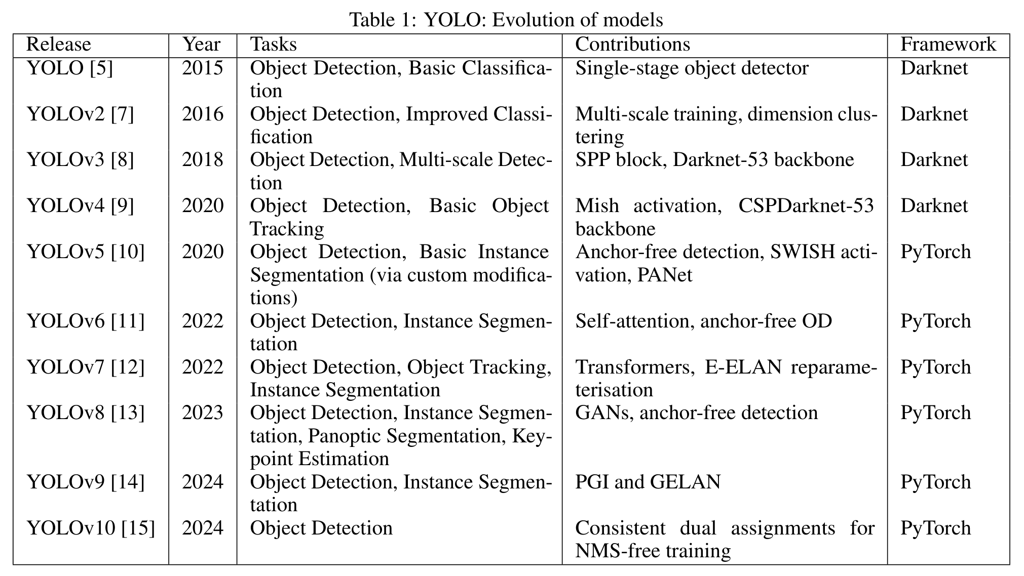
The paper's Table 1 traces that argument version by version. YOLOv2 added multi-scale training and dimension-clustered anchors; YOLOv3 brought the Darknet-53 backbone, multi-scale prediction and an SPP block; YOLOv4 moved to CSPDarknet-53 with Mish activations. YOLOv5 marked the jump from Darknet to PyTorch, and with YOLOv8 (2023) Ultralytics settled on the anchor-free, multi-task design YOLO11 extends. 2024 alone produced three releases: YOLOv9 (Programmable Gradient Information and GELAN), YOLOv10 (consistent dual assignments for NMS-free training) and YOLO11.
The table is a compressed summary and some of its one-line attributions are loose — YOLOv5's official detector, for instance, is anchor-based, and anchor-free heads became the Ultralytics default with YOLOv8. What matters for YOLO11 is the immediate parent: it is an evolution of YOLOv8, not of YOLOv10. It keeps YOLOv8's backbone/neck/head topology and task heads, swaps C2f for C3k2, and borrows the idea of a lightweight attention block at the coarsest scale — an idea YOLOv10 had also used in its PSA module.
Key Points
YOLO (2015) reframed detection as a single regression problem: one CNN predicts boxes and class probabilities for the entire image in one pass
YOLOv2–v4 stayed on Darknet: multi-scale training and dimension clustering (v2), Darknet-53 + SPP (v3), CSPDarknet-53 + Mish (v4)
YOLOv5 (2020) moved the series to PyTorch; every version since in the table is PyTorch-based
YOLOv8 (2023) introduced the anchor-free, multi-task Ultralytics design — detection, segmentation and keypoints from one codebase
2024 releases: YOLOv9 (PGI + GELAN), YOLOv10 (consistent dual assignments → NMS-free), then YOLO11
YOLO11 builds directly on YOLOv8 — the paper repeatedly frames its changes as modifications of YOLOv8's blocks
Unlike most YOLOs, YOLO11 shipped as code from Ultralytics; this paper is an after-the-fact architectural analysis of that release
Every YOLO has the same three-stage shape, and YOLO11 does not change it. The backbone is a stack of strided convolutions and specialised blocks that turns a raw image into feature maps at several resolutions. The neck aggregates those maps across scales — upsampling coarse, semantic features and concatenating them with fine, spatially precise ones. The head turns each fused map into predictions.
Because the whole network is one differentiable graph, box regression and classification are trained end-to-end — the property that separated YOLO from two-stage detectors in the first place. What YOLO11 changes is which blocks fill the stages. In the backbone, initial strided convolutions downsample the image while widening channels, and the C3k2 block replaces YOLOv8's C2f. At the bottom of the backbone the SPPF block is retained and a new C2PSA block follows it. In the neck, C3k2 again replaces C2f after each upsample-and-concatenate step. And in the head, multiple C3k2 blocks and CBS (Conv-BatchNorm-SiLU) layers refine features before the final Conv2D branches.
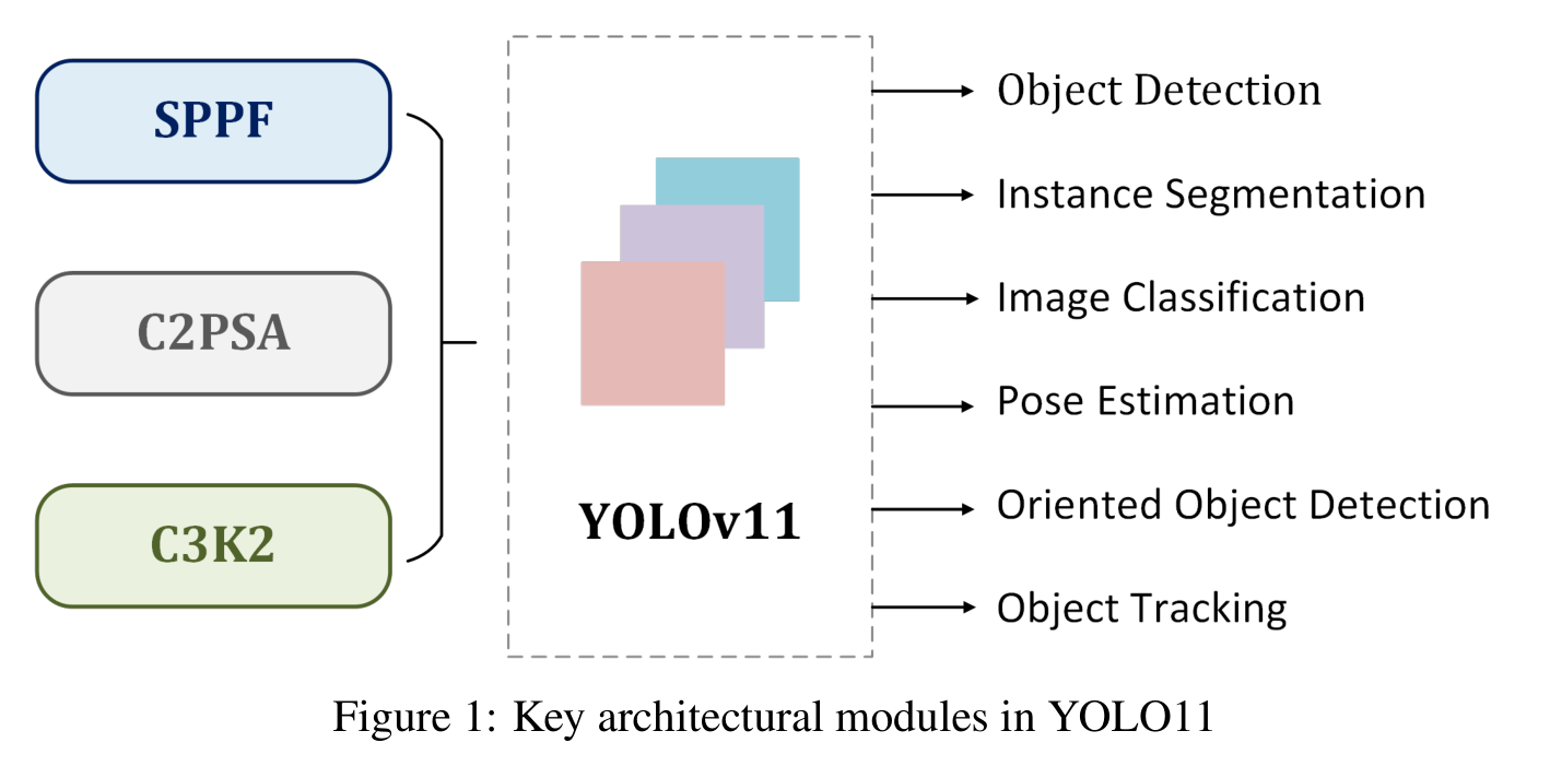
The paper's Figure 1 compresses this into one picture: three key modules — SPPF, C2PSA, C3k2 — feeding one model that serves six task types. The scale structure is worth internalising concretely. With the standard 640×640 input, the head reads features at strides 8, 16 and 32 — grids of 80×80, 40×40 and 20×20 — so small objects are predicted from the fine map and large objects from the coarse one. C2PSA sits on that coarsest 20×20 map, which is exactly where attention is affordable.
Key Points
Backbone — feature extraction at multiple scales: strided convolutions downsample while increasing channels; C3k2 replaces C2f
End of backbone — SPPF is kept from earlier versions; C2PSA is newly inserted right after it
Neck — upsampling + concatenation across levels, with C3k2 after each fusion step instead of C2f
Head — multiple C3k2 blocks and CBS layers refine features; per-branch Conv2D layers produce the final outputs
Three prediction scales at strides 8 / 16 / 32 — for a 640×640 input, grids of 80×80, 40×40, 20×20
YOLO11 extends YOLOv8's layout rather than redesigning it: the innovation is in the blocks, not the topology
Mathematical Formulation
Feature-map size per prediction scale
Each backbone downsampling step halves the resolution. The head reads three of these levels: stride 8 (P3) for small objects, stride 16 (P4) for medium, stride 32 (P5) for large. The P5 map is where SPPF and C2PSA operate.
The workhorse of YOLO11 is the C3k2 block, and it appears everywhere: backbone, neck and head. It replaces YOLOv8's C2f, and both are descendants of the Cross Stage Partial (CSP) idea — split the channels, send only part of them through the expensive transformation, and merge everything back at the end. The untouched part keeps a cheap gradient path and avoids recomputing redundant features; the transformed part does the real work.
The paper describes C3k2 as a more computationally efficient CSP bottleneck that uses two smaller convolutions instead of one large convolution. That trade is classic: two stacked 3×3 convolutions cover the same 5×5 receptive field as one 5×5 convolution, with fewer weights and an extra non-linearity in between. The paper reads the "k2" in the name as signalling this smaller-kernel design, and attributes C3k2's speed to it.
The interesting part is the c3k switch. With c3k = False, C3k2 behaves like C2f: its inner units are standard bottlenecks. With c3k = True, each inner bottleneck is replaced by a C3k module — a C3-style block whose kernel size is customisable — allowing deeper, more complex feature extraction. In the Ultralytics configuration, the shallow, high-resolution stages run the cheap variant and the deeper stages turn C3k on, spending capacity where the feature maps are small. Under the hood (Ultralytics implementation), C3k2 inherits C2f's "split and keep every intermediate" wiring: a 1×1 conv produces two halves, each inner module's output is appended to the running list, and a final 1×1 conv fuses the concatenation.
Key Points
Replaces C2f from YOLOv8 in the backbone, the neck and the head
A more compact Cross Stage Partial (CSP) bottleneck: part of the channels bypass the heavy path, the rest are transformed, then all are concatenated
Two smaller convolutions instead of one large one — lower compute for a comparable receptive field
c3k = False → behaves like C2f with standard bottleneck units
c3k = True → inner bottlenecks become C3k modules (customisable kernel size) for deeper feature extraction
Paper-stated benefits: faster processing and parameter efficiency — fewer trainable parameters than the CSP block it replaces
Mathematical Formulation
Why two small kernels beat one large one
Two stacked convolutions see the same input window as a single convolution, but with 28% fewer weights for input and output channels — and an extra activation between them. This is the efficiency argument behind "two smaller convolutions".
Channel accounting (C2f-style wiring)
Each of the inner modules (a bottleneck, or a C3k module when is true) takes the previous output and adds one more -channel tensor to the list, so the final conv fuses channels. This follows the Ultralytics implementation that C3k2 inherits from C2f.
At the bottom of the backbone the feature map is small (20×20 for a 640 input) but each cell must reason about objects that may span most of the image. Spatial Pyramid Pooling solves this by max-pooling the same map at several window sizes and concatenating the results, so every position carries summaries of its neighbourhood at multiple scales. YOLOv3 brought an SPP block into the series; YOLO11 retains the fast variant, SPPF, from previous versions.
The "fast" part is a neat identity. The original SPP block pools the input in parallel with 5×5, 9×9 and 13×13 windows. But stride-1 max-pooling composes: pooling a 5×5-pooled map again with a 5×5 window is exactly a 9×9 max-pool, and doing it a third time gives 13×13. So SPPF runs one 5×5 max-pool three times in sequence and concatenates the input with all three intermediate outputs — the same multi-scale features, computed by reusing work instead of re-scanning large windows.
In YOLO11, SPPF is no longer the last word at the bottom of the backbone: its output feeds directly into the new C2PSA block. SPPF supplies fixed, hand-designed multi-scale context; C2PSA then adds learned, content-dependent context through attention.
Key Points
Retained from earlier YOLO versions — YOLO11 keeps SPPF at the end of the backbone
Multi-scale context: each output position summarises its neighbourhood at several window sizes
SPPF chains three 5×5 stride-1 max-pools; their receptive fields are 5, 9 and 13 — matching the parallel 5/9/13 pools of classic SPP
The input and all three pooled maps are concatenated and fused by a 1×1 convolution (Ultralytics implementation)
Faster than parallel SPP because each pool reuses the previous result instead of scanning a large window
Its output feeds the new C2PSA block, which adds learned spatial attention on top of fixed pooling
Mathematical Formulation
SPPF as sequential pooling
is a max-pool with stride 1 and padding 2, so spatial size is preserved and the four maps can be concatenated channel-wise.
Why it equals SPP(5, 9, 13)
A max over a max is a max over the union of the windows. Two stacked windows with stride 1 cover a window (); three cover . The result is identical to parallel SPP, at lower cost.
Convolutions and pooling are local and content-blind: a 5×5 kernel weighs its neighbours the same way regardless of what is in the image. The genuinely new block in YOLO11 is C2PSA, which the paper describes as a Cross Stage Partial block with spatial attention (the abstract expands it as "Convolutional block with Parallel Spatial Attention"). It is inserted immediately after SPPF at the end of the backbone.
Its job, per the paper, is to let the model focus on important regions of the feature map. Attention computes, for every spatial position, a weighted mix of every other position, with weights derived from the content itself — so a cell on a partly occluded object can draw evidence from distant cells on the visible parts. The paper argues this is especially useful for smaller or partially occluded objects, and singles C2PSA out as a key difference from YOLOv8, which has no such mechanism.
Two design choices keep it real-time. First, placement: self-attention costs grow with the square of the number of positions, so the block lives on the coarsest map (20×20 = 400 positions at 640 input) rather than the 80×80 map. Second, the CSP wrapper — in the Ultralytics implementation the input is projected and split in two; only one half passes through the position-sensitive attention (PSA) blocks, each an attention layer followed by a feed-forward layer with residual connections, and the halves are concatenated and fused by a 1×1 conv. Half the channels see attention; the other half carry the SPPF features through untouched.
Key Points
New in YOLO11 — placed directly after SPPF at the end of the backbone
Spatial attention: each position aggregates information from all other positions, weighted by content similarity
Paper's motivation: concentrate on regions of interest, improving detection of objects of varying sizes and positions, especially small or partially occluded ones
YOLOv8 lacks this mechanism — the paper names C2PSA as a defining difference between the two
Runs on the coarsest (stride-32) map, where the quadratic cost of attention is affordable
A CSP split (Ultralytics implementation) sends only half the channels through attention + FFN, then concatenates both halves
Mathematical Formulation
Self-attention over spatial positions
The feature map is flattened into tokens. Each row of the softmax matrix says how much one position attends to every other — the "focus on important regions" the paper describes.
Why only at stride 32
The attention matrix has entries. On the P5 map that is 160K pairs; on the P3 map it would be 256 times more. Placing C2PSA at the end of the backbone buys global context at a cost a real-time detector can afford.
The head receives three fused maps from the neck and must turn each into concrete predictions. YOLO11 first refines them: multiple C3k2 blocks process the multi-scale features at different depths, followed by CBS layers — a convolution, then batch normalisation, then a SiLU activation.
Each piece of CBS has a distinct role in the paper's description. The convolution extracts the features relevant to detection; batch normalisation stabilises and normalises the data flow, keeping activations in a well-conditioned range so training is stable; and SiLU supplies the non-linearity. SiLU, , is smooth and non-monotonic — unlike ReLU it lets small negative values through, which tends to help deep detectors train.
Finally, each detection branch ends in a set of Conv2D layers that reduce the features to exactly the number of outputs required, and a Detect layer consolidates them. The paper lists three output types: bounding-box coordinates for localisation, objectness scores, and class scores. One caveat worth knowing when you read the Ultralytics code: since YOLOv8 the head is anchor-free and decoupled, with a box-regression branch and a classification branch, and no separate objectness output — the class scores themselves play that role. Every grid cell on every scale makes a prediction, so a 640×640 image yields 8,400 candidate boxes before post-processing.
Key Points
The head uses multiple C3k2 blocks in several pathways to process features at different depths
CBS = Conv → BatchNorm → SiLU, applied after the C3k2 blocks
Conv extracts relevant features; BatchNorm stabilises and normalises the data flow; SiLU adds non-linearity
Each branch ends with Conv2D layers that map features to the exact number of outputs needed
The Detect layer consolidates box coordinates and class scores (the paper also lists objectness scores)
In the Ultralytics implementation the head is anchor-free and decoupled — box and class branches are separate
Predictions are dense: 8,400 candidates for a 640×640 input across the three scales
Mathematical Formulation
The CBS block
Convolution , batch normalisation, then the Sigmoid Linear Unit. SiLU is smooth everywhere and dips slightly below zero for negative inputs before returning to zero, rather than clipping hard as ReLU does.
Dense predictions across three scales
Each cell of each prediction grid emits one box and a vector of class scores; low-confidence and duplicate candidates are filtered afterwards.
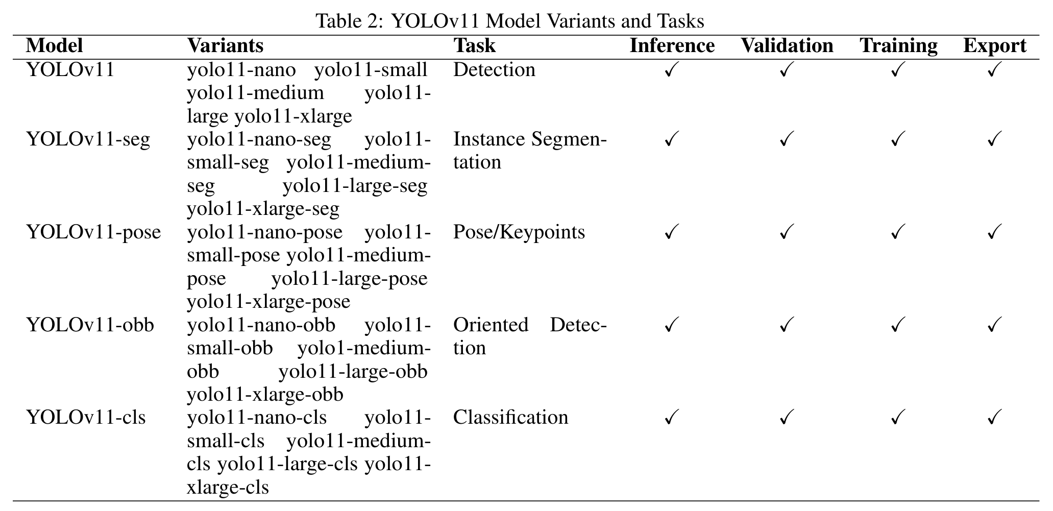
The broadest change from earlier YOLOs is not a block but a product decision: YOLO11 is a family of task-specific models sharing one backbone and neck design. The paper's Table 2 lists five variants — YOLOv11 (detection), -seg (instance segmentation), -pose (pose/keypoints), -obb (oriented detection) and -cls (classification) — each available in nano, small, medium, large and extra-large sizes, and every one supporting inference, validation, training and export.
The tasks differ only in what the head emits. Detection outputs axis-aligned boxes and classes. Instance segmentation goes to pixel level, separating individual objects — the paper points to medical imaging and manufacturing defect inspection. Pose estimation predicts keypoints for movement tracking in fitness, sports and healthcare. Oriented object detection adds an angle to each box so rotated objects are tightly enclosed — valuable in aerial imagery, robotics and warehouses. Classification assigns one label to the whole image. Object tracking — the sixth capability in Figure 1 — links detections across video frames.
Why is this cheap? Because the expensive part — learning good multi-scale features — is shared. A segmentation or pose model is the same feature extractor with a different final layer, so architectural improvements like C3k2 and C2PSA lift every task at once. And the n-to-x size ladder lets the same design target an edge device or a GPU server.
Key Points
Object detection — boxes and classes; surveillance, autonomous vehicles, retail analytics
Instance segmentation — per-object pixel masks; medical imaging, manufacturing defect detection
Image classification — one label per image; e-commerce categorisation, wildlife monitoring
Pose estimation — keypoints; fitness tracking, sports analysis, healthcare motion assessment
Oriented object detection (OBB) — boxes with an angle; aerial imagery, robotics, warehouse automation
Object tracking — follows objects across frames; traffic monitoring, security
Each task ships in five sizes (n, s, m, l, x), all supporting inference, validation, training and export (Table 2)
Mathematical Formulation
From axis-aligned to oriented boxes
An oriented bounding box adds a rotation angle , so a ship or a vehicle seen from above at 30° is enclosed tightly instead of by a large axis-aligned rectangle full of background.
The paper's evidence is Ultralytics' published benchmark (its reference [23]), reproduced as Figure 2: COCO mAP against latency on a T4 GPU with TensorRT FP16, for YOLOv5 through YOLOv10, PP-YOLOE+ and YOLO11. The authors do not run new experiments, so these are the vendor's numbers — but the comparison is like-for-like on hardware and dataset.
The YOLO11 variants (11n, 11s, 11m, 11l, 11x) form a distinct frontier: at each latency point they reach a higher mAP than earlier versions. The paper highlights YOLO11x at roughly 54.5% mAP and about 13 ms, above every previous YOLO, and YOLO11s at about 47% in the 2–6 ms low-latency regime — accuracy previously reserved for much slower models. YOLO11m reaches accuracy comparable to larger previous-generation models in significantly less time.
The cleanest single number is parameter efficiency: YOLO11m achieves higher COCO mAP than YOLOv8m with 22% fewer parameters. The paper ties this back to the architecture — C3k2's compact CSP design trims parameters, while C2PSA and SPPF improve feature quality. It also notes that the nano model, despite a slight increase in parameters over its predecessor, improves inference speed and FPS. The honest limitation is that no ablation isolates each block: the gains are measured for the whole model, so how much is due to C3k2, C2PSA or training changes is not separated.
Key Points
Benchmark: COCO mAP vs. T4 TensorRT FP16 latency, from Ultralytics' documentation (paper ref. [23])
YOLO11 n/s/m/l/x form a Pareto frontier above YOLOv5–v10 and PP-YOLOE+
YOLO11x ≈ 54.5% mAP at ≈ 13 ms — the highest of any YOLO in the comparison
YOLO11s ≈ 47% mAP in the 2–6 ms low-latency regime
YOLO11m: higher mAP than YOLOv8m with 22% fewer parameters
The nano model gains inference speed and FPS over its predecessor despite slightly more parameters
No per-block ablation: results are for the full model, so individual contributions of C3k2 / C2PSA are not isolated
Mathematical Formulation
COCO mAP over IoU thresholds
Average precision is averaged over classes and over ten IoU thresholds, so a model only scores well if its boxes are tight — a loose box that counts at IoU 0.5 fails at 0.75 and above.
Parameter efficiency vs. YOLOv8m
Fewer parameters and higher accuracy at the same time — the paper's central quantitative claim for the architectural changes.