InternVL3.5
Advancing Open-Source Multimodal Models in Versatility, Reasoning, and Efficiency
Weiyun Wang, Zhangwei Gao, Lixin Gu, Hengjun Pu, Long Cui, Xingguang Wei,
9
Concepts
14
Formulas
13
Figures
5
Demos
Paper Overview
InternVL3.5 (Wang, Gao, Gu et al. — InternVL Team, Shanghai AI Laboratory, 2025) is an open family of multimodal models from 1B to 241B parameters, dense and mixture-of-experts. Its main argument is about recipes rather than architecture. The model keeps the familiar ViT–MLP–LLM layout, and the paper attributes its gains to three changes in how the model is trained and served.
The first is Cascade RL. Offline RL (MPO) is cheap and stable but plateaus early, while online RL (GSPO) climbs higher but is expensive and fragile from a weak start. Running MPO first as a warm-up and GSPO second as a refinement gives the 8B model 60.3 on a seven-benchmark reasoning suite. Two full episodes of GSPO alone reach 58.2 while using about twice the GPU hours.
The second and third target inference cost. A Visual Resolution Router (ViR), trained through Visual Consistency Learning (ViCO), decides per image patch whether 64 visual tokens are enough or 256 are needed, which halves visual tokens at almost no loss in accuracy. Decoupled Vision-Language Deployment (DvD) runs the vision encoder and the LLM on separate servers in an asynchronous pipeline so neither blocks the other. Together they give up to 4.05x request throughput over the baseline.
The paper reports up to +16.0% overall reasoning over InternVL3, 77.7 on MMMU for the 241B-A28B flagship, a general-multimodal score of 74.1 vs GPT-5's 74.0, and new capabilities in GUI control, embodied spatial reasoning and SVG generation, with all weights released.
Chapter Roadmap
Click any topic to jump in
The Open-Source Gap
Reasoning, text and agentic tasks are where open MLLMs trail. Unstable RL and rising visual-token cost are the two obstacles.
ViT–MLP–LLM Family
InternViT + Qwen3/GPT-OSS, nine sizes from 1B to 241B-A28B. Dynamic tiling with 256 tokens per tile after pixel shuffle.
Native Pre-Training + SFT
~250B tokens of joint text + multimodal pre-training, then ~130B tokens of SFT with Thinking-mode and agentic data.
Reasoning and efficiency
Cascade RL
Offline MPO warm-up, then online GSPO: 60.3 vs 58.2 for two GSPO episodes, at about half the GPU hours.
ViR + ViCO
A per-patch router picks 64 or 256 tokens, trained by consistency KL then self-labelled loss ratios. 50% fewer tokens.
Inference-time compute and serving
Test-Time Scaling
Thinking mode for depth plus Best-of-N with VisualPRM for breadth. Applied to reasoning tasks only.
Decoupled Deployment
ViT and LLM on separate servers in an async pipeline: up to 2.01x alone and 4.05x with ViR.
Outcomes
Results
74.1 vs GPT-5's 74.0 on general tasks, 77.7 MMMU, and Cascade RL gains at every scale.
GUI, Embodied, SVG
92.9 ScreenSpot-v2, 69.5 VSI-Bench and 70.7 SGP-Bench: one open model across agentic domains.
Concept by concept
9 sections, in reading order.
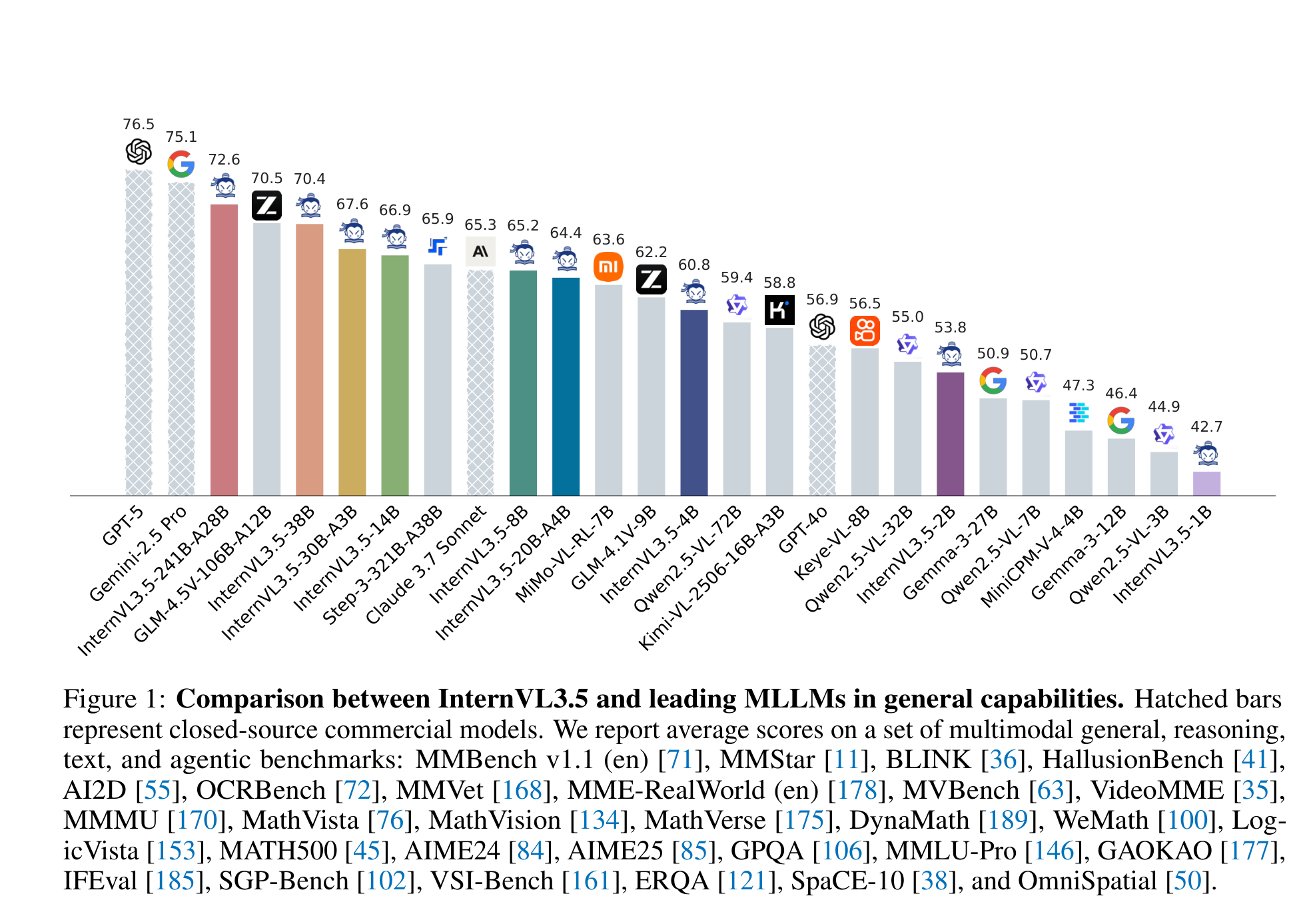
By mid-2025 multimodal models were no longer judged on describing pictures. The tasks that mattered had moved to reasoning (MMMU, MathVista), text-heavy work (AIME, GPQA, MMLU-Pro) and agentic behaviour (GUI control, embodied spatial reasoning). On those, commercial models had opened a wide lead over open-source ones, and the InternVL team frames InternVL3.5 as an attempt to close it.
The paper names two obstacles. The first is reinforcement learning. Open-source groups had been applying RL to MLLMs to buy reasoning, but in the paper's words a stable, effective, and scalable RL framework for MLLMs was still an open problem. Offline methods such as DPO are cheap and stable but have a lower ceiling; online methods such as PPO or GRPO reach higher but cost far more GPU time and are touchier to train.
The second obstacle is cost at inference. High-resolution understanding, multi-image input and long video all multiply the number of visual tokens, and each extra token makes deployment slower. The capabilities that close the quality gap widen the cost gap.
InternVL3.5 answers each obstacle with its own mechanism. Cascade RL runs offline RL as a warm-up and then online RL as a refinement, aimed at reasoning. A Visual Resolution Router (ViR) decides per image patch how hard the visual tokens can be compressed, and Decoupled Vision-Language Deployment (DvD) puts the vision encoder and the LLM on separate GPUs so they stop blocking each other. Both target efficiency. Against InternVL3 the paper reports up to +16.0% overall reasoning performance and a 4.05x inference speed-up. Against GPT-5, the flagship InternVL3.5-241B-A28B narrows the overall gap to 3.9%.
Key Points
- 1
Frontier MLLM evaluation has shifted to reasoning, text and agentic tasks, where commercial models led open-source ones by wide margins
- 2
Open problem #1: no stable, effective, scalable RL recipe for MLLMs. Offline RL (DPO-style) is cheap but has a low ceiling, while online RL is strong but expensive
- 3
Open problem #2: high-resolution, multi-image and video inputs multiply visual tokens, which drives up inference cost
- 4
Three proposals: Cascade RL for reasoning, plus ViR and DvD for efficiency
- 5
Headline vs InternVL3: up to +16.0% overall reasoning and 4.05x inference speed-up
- 6
InternVL3.5-241B-A28B narrows the overall gap to GPT-5 to 3.9%, and on general multimodal tasks scores 74.1 vs 74.0 (Table 2)
- 7
Every model from 1B to 241B, dense and MoE, is released with code
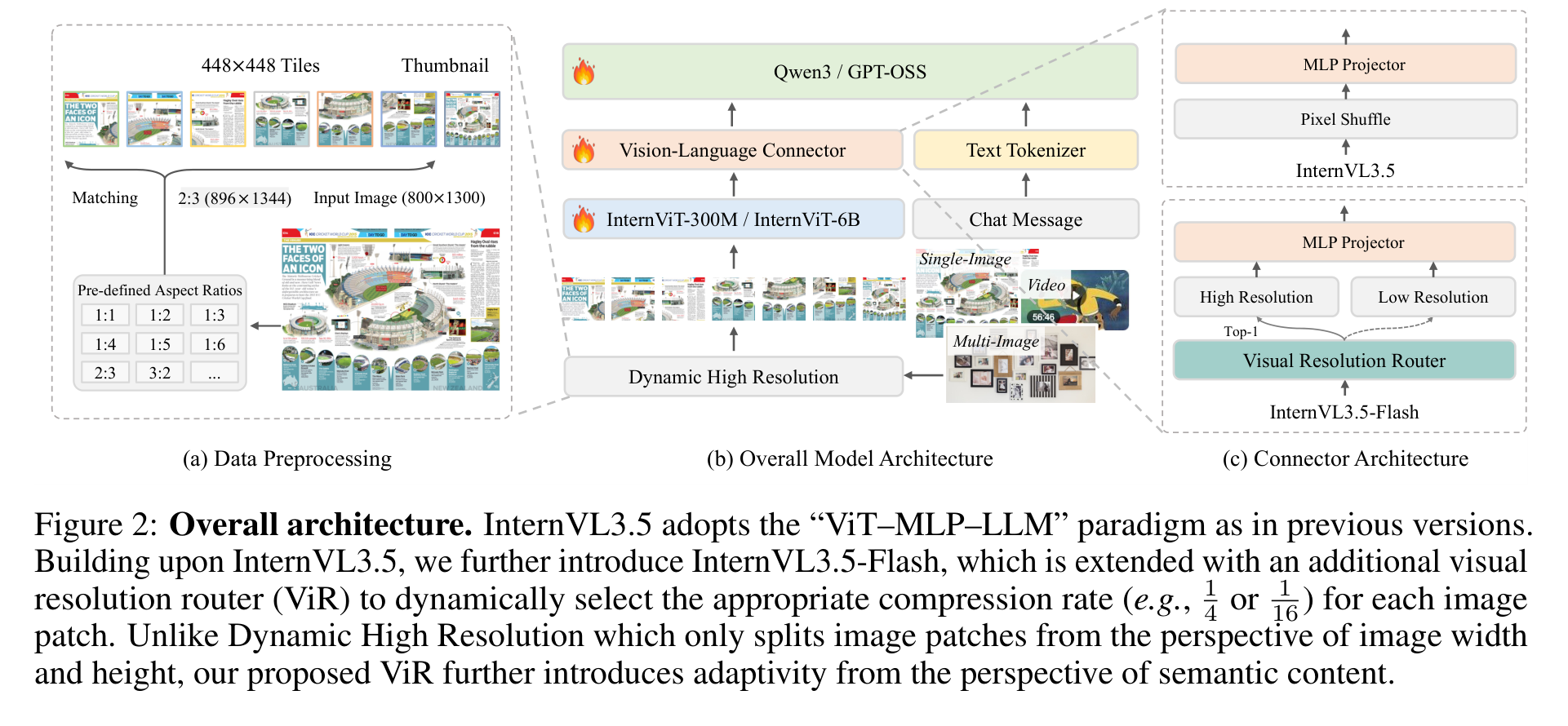
The architecture is deliberately unchanged. InternVL3.5 keeps the ViT–MLP–LLM layout used by earlier InternVL versions. A vision transformer encodes the image, an MLP projector maps its features into the language model's embedding space, and the LLM does the rest. Every gain the paper reports therefore comes from training, routing and serving rather than a new backbone.
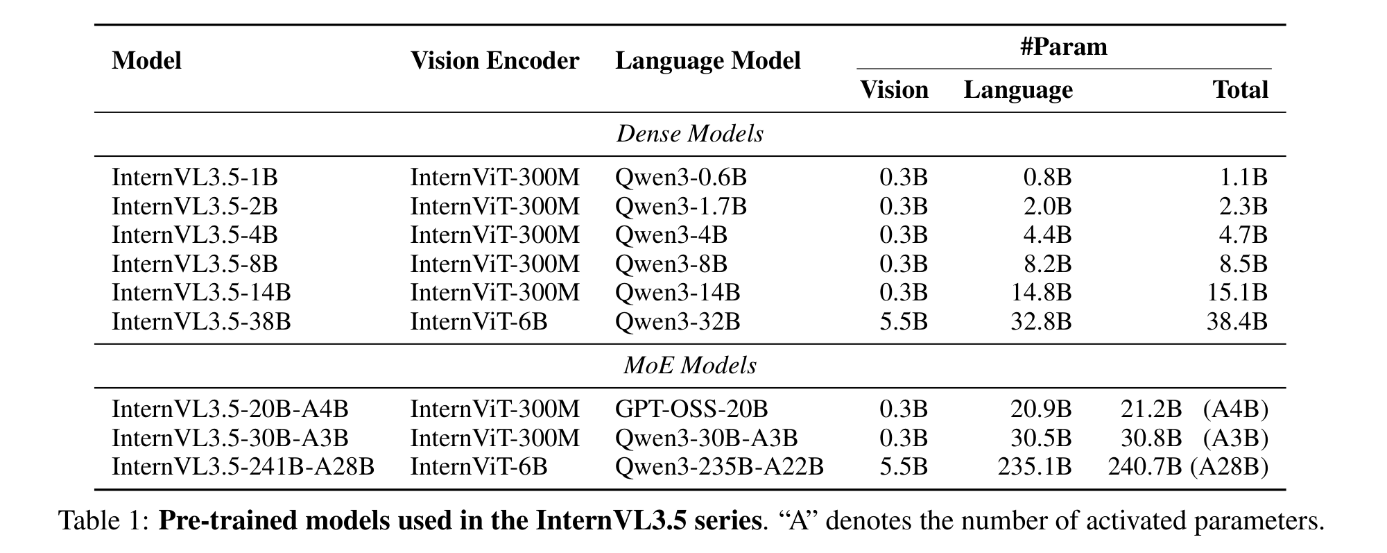
What changes is the components. The language side is initialised from Qwen3 (0.6B up to the 235B-A22B MoE) and, for one variant, GPT-OSS-20B. The vision side is InternViT-300M for most sizes and InternViT-6B for the 38B and 241B models. The result is nine models, from InternVL3.5-1B (1.1B total) to InternVL3.5-241B-A28B, which has 240.7B parameters but activates only 28B per token.
Images enter through Dynamic High Resolution, inherited from InternVL1.5. An image is matched to the closest of a set of predefined aspect ratios, resized, cut into 448×448 tiles, and given a downscaled thumbnail for global context. An 800×1300 image, for example, matches the 2:3 ratio and becomes a 896×1344 grid of six tiles plus the thumbnail. Each tile becomes 1024 ViT tokens, and a pixel shuffle folds every 2×2 neighbourhood into the channel dimension, which leaves 256 tokens per tile for the LLM.
Dynamic High Resolution adapts to an image's shape: wide images get wide grids. It does not adapt to content. A tile of blank sky costs the same 256 tokens as a tile of dense small print. InternVL3.5-Flash adds the Visual Resolution Router to close that gap (see the ViR section).
Key Points
- 1
Same ViT–MLP–LLM paradigm as earlier InternVL versions; the gains come from training and serving, not a new layout
- 2
LLM initialised from Qwen3 (0.6B–235B-A22B) or GPT-OSS-20B; vision encoder is InternViT-300M or InternViT-6B
- 3
Nine sizes: six dense (1B, 2B, 4B, 8B, 14B, 38B) and three MoE (20B-A4B, 30B-A3B, 241B-A28B). The 241B-A28B model has 240.7B total and 28B activated parameters
- 4
Dynamic High Resolution: match the closest predefined aspect ratio, tile into 448×448 patches, and add a thumbnail for global context
- 5
Each tile is 1024 ViT tokens, compressed by pixel shuffle to 256 tokens before the LLM
- 6
Tiling adapts to image shape, not content. Closing that gap is what the ViR in InternVL3.5-Flash is for
Mathematical Formulation
Pixel Shuffle Token Budget
1024 ViT tokens32×32 pixel shuffle (2×2) 256 LLM tokens16×16,ξ=1024256=41
Pixel shuffle trades spatial resolution for channel depth: every 2×2 block of ViT features is concatenated into one token. The paper calls this a compression rate of ξ=41. InternVL3.5-Flash adds a second, more aggressive shuffle with ξ=161 (64 tokens per tile).
Visual Tokens for a Tiled Image
Nvis=(ntiles+1)×256
The +1 is the thumbnail. The paper's 800×1300 example matches the 2:3 ratio (896×1344), giving ntiles=6 and Nvis=7×256=1792 visual tokens before any routing.
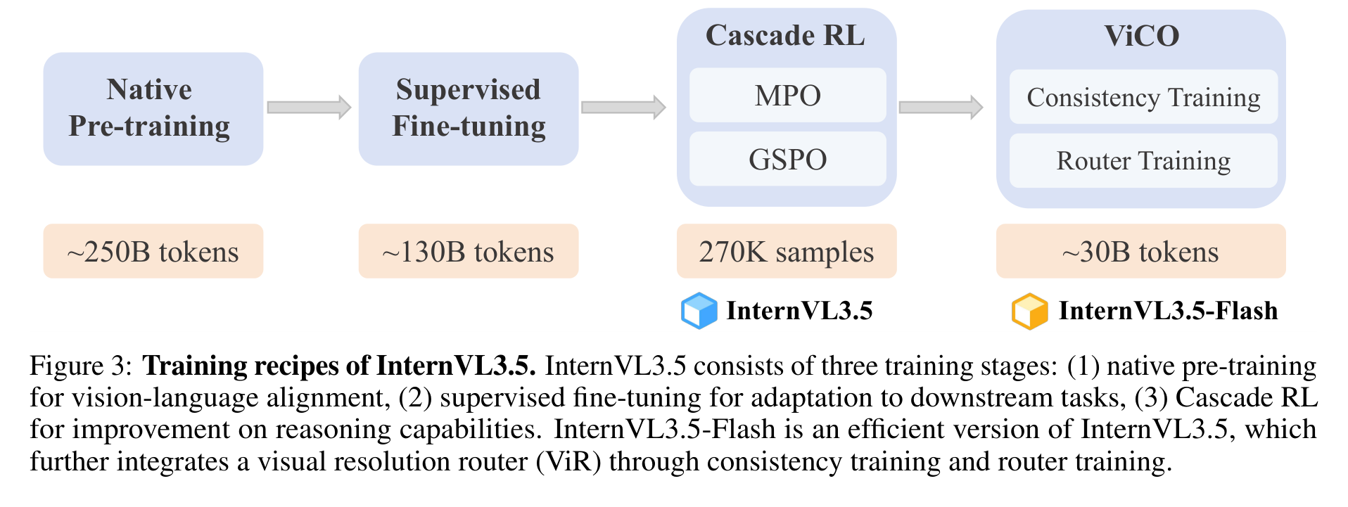
Before any RL, InternVL3.5 goes through two supervised stages that both use next-token prediction on text tokens.
Native pre-training updates all parameters jointly on a mix of multimodal and text-only data. The vision encoder, projector and LLM are not frozen, and there is no separate alignment warm-up. The corpus is about 116M samples / 250B tokens with a text-only to multimodal ratio of roughly 1 : 2.5, at a maximum sequence length of 32K. The large share of pure text is deliberate. The paper credits this native strategy, introduced in InternVL3, with preserving the LLM's language ability and avoiding the catastrophic forgetting that hurts vision-language models whose LLM forgets how to do maths once it learns to see.
A quieter design choice concerns how the loss is averaged. If every token gets equal weight, long responses dominate the gradient. If every sample gets equal weight, a 5-token answer counts as much as a 2,000-token derivation. InternVL3.5 uses square averaging: each token is weighted by 1/N0.5, where N is the number of loss tokens in its sample. This sits between the two extremes and counters bias toward either longer or shorter responses. Random JPEG compression is also applied as augmentation for real-world robustness.
Supervised fine-tuning keeps the same objective but switches to higher-quality conversation data: about 56M samples / 130B tokens (text to multimodal about 1 : 3.5), again at 32K context. The data comes from three sources. The first is InternVL3's instruction data, kept for coverage. The second is "Thinking"-mode reasoning data, sampled from a large reasoning model and filtered for correctness as well as for the clarity, redundancy and formatting of the reasoning itself. The third is capability-expansion data for GUI interaction, embodied interaction, and SVG understanding and generation. Most of the agentic results trace back to this third source.
Key Points
- 1
Three training stages for InternVL3.5: native pre-training → SFT → Cascade RL. InternVL3.5-Flash adds ViCO on top
- 2
Pre-training updates all parameters jointly on ~116M samples / ~250B tokens, text-only : multimodal ≈ 1 : 2.5, max length 32K
- 3
Loss is computed only on text tokens (only response tokens for conversations); image tokens act purely as context
- 4
Square averaging weights each token by 1/N0.5 to avoid bias toward long or short responses
- 5
SFT: ~56M samples / ~130B tokens, text-only : multimodal ≈ 1 : 3.5, 32K context
- 6
SFT data = InternVL3 instruction data + filtered Thinking-mode reasoning traces + capability-expansion data (GUI, embodied, SVG)
- 7
The paper credits the large text-only share with preserving language skills: InternVL3.5-1B beats its own Qwen3-0.6B base on 15 of 16 text benchmarks (+6.7 overall)
Mathematical Formulation
Next-Token Prediction Loss
Li=−logpθ(xi∣x1,…,xi−1)
Computed on each text token xi. The prefix may contain both text and image tokens, so the image conditions the prediction but is never itself a prediction target.
Square-Averaged Loss Weighting
Li′=∑jwjwi⋅Li,wi=N0.51
N is the number of loss-bearing tokens in the sample. Token averaging (w=1) favours long samples, and sample averaging (w=1/N) favours short ones. The square root splits the difference.
Supervised learning only shows the model good answers. RL's main advantage, in the paper's framing, is that it brings in negative samples that prune low-quality regions of the output space. The open question is which kind of RL to use.
Offline RL (DPO-style methods, which train on a fixed set of pre-collected rollouts) is efficient and stable, because collecting rollouts and updating parameters are decoupled, which also blunts reward hacking. Its ceiling is lower. Online RL (PPO, GRPO, GSPO, which sample fresh rollouts from the current policy) reaches higher but is expensive, and it only works well if the model already produces good-enough rollouts to learn from.
Cascade RL chains the two. Stage one is MPO (Mixed Preference Optimization), an offline method whose loss combines a DPO preference term, a BCO quality term and a plain LM generation term. It runs on MMPR-v1.2 (about 200K preference pairs) and serves as a cheap warm-up that lifts the model to the point where its own rollouts are high quality. Stage two is GSPO (Group Sequence Policy Optimization), online and without a reference-model constraint. GSPO normalises rewards within a group of sampled responses, as GRPO does, but computes the importance ratio at the sequence level as a length-normalised geometric mean of per-token ratios. The paper finds this more effective for both dense and MoE models. Online data is MMPR-Tiny, about 70K queries, chosen where the model's accuracy lies between 0.2 and 0.8 so every prompt carries learning signal. The MMPR-v1.2 rollouts are reused for both the offline stage and this filtering, so no extra sampling is needed.
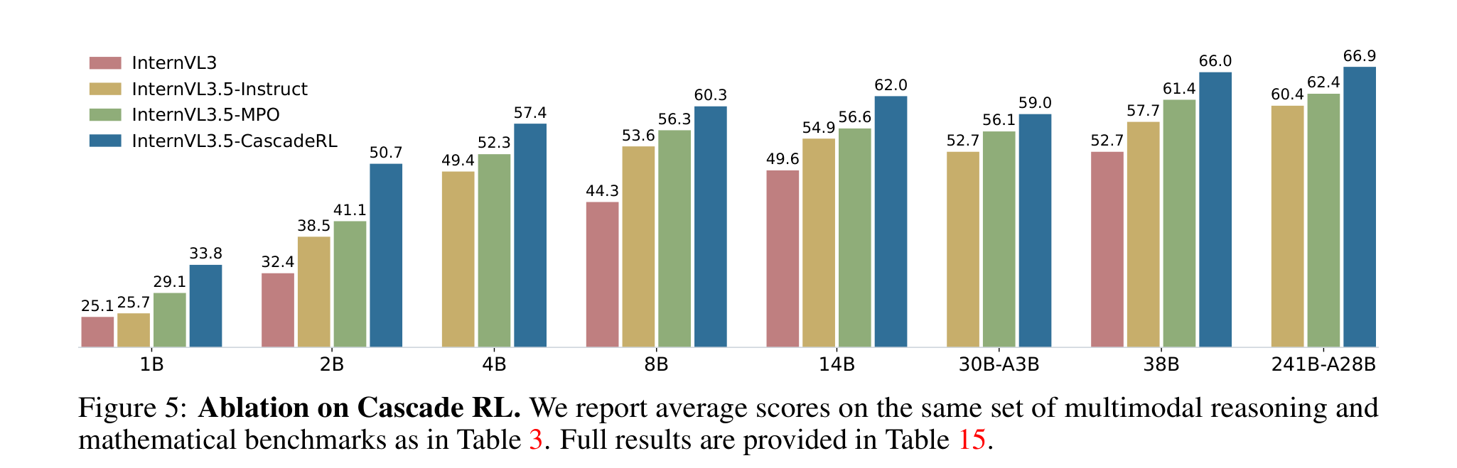
The ablation in Table 16 (8B model) shows the economics. MPO alone takes about 0.3K GPU hours to reach 56.3. GSPO alone takes about 5.5K hours for 57.3, and doubling to about 11.0K hours reaches only 58.2. Cascade RL uses about 5.8K hours and reaches 60.3. That is better than twice the GSPO budget at roughly half its cost. The warm-up does more than save compute: a stronger starting policy makes the online stage more stable and lets it climb higher in fewer steps.

Key Points
- 1
RL's core advantage over SFT: negative samples prune low-quality regions of the model's output space
- 2
Offline RL (DPO family) is efficient and stable but has a lower ceiling. Online RL (PPO/GRPO/GSPO) reaches higher but is costly and needs good rollouts
- 3
Stage 1, MPO: LMPO=wpLp+wqLq+wgLg with DPO, BCO and LM losses, trained on MMPR-v1.2 (~200K pairs)
- 4
Stage 2, GSPO without a reference-model constraint: group-normalised advantages with a sequence-level importance ratio, trained on MMPR-Tiny (~70K queries with accuracy in 0.2–0.8)
- 5
Advantages claimed: stability (offline decoupling resists reward hacking, and a stronger start stabilises the online stage), efficiency (rollouts shared across models) and a higher ceiling
- 6
Table 16 (8B): Instruct 53.6 → MPO 56.3 (~0.3K h) | GSPO 1 ep 57.3 (~5.5K h) | GSPO 2 ep 58.2 (~11.0K h) | Cascade RL 60.3 (~5.8K h)
- 7
Cascade RL beats two full GSPO episodes using about half the GPU hours
Mathematical Formulation
MPO — The Offline Stage
LMPO=wpLp+wqLq+wgLg
Lp is the DPO preference loss (chosen beats rejected), Lq the BCO quality loss (each response judged good or bad on its own), and Lg the ordinary LM loss on chosen responses, which keeps generation fluent.
Group-Normalised Advantage
A^i=std({r(x,yi)}i=1G)r(x,yi)−mean({r(x,yi)}i=1G)
For each query x, G responses are sampled and each reward is standardised against its own group, as in GRPO. No value network is needed, because the group itself is the baseline.
GSPO Objective
LGSPO(θ)=Ex∼D,{yi}i=1G∼πθold(⋅∣x)[G1∑i=1Gmin(si(θ)A^i,clip(si(θ),1−ε,1+ε)A^i)]
A PPO-style clipped surrogate, except that clipping is applied once per response using the sequence-level ratio si(θ), rather than once per token.
Sequence-Level Importance Ratio
si(θ)=(πθold(yi∣x)πθ(yi∣x))∣yi∣1=exp(∣yi∣1∑t=1∣yi∣logπθold(yi,t∣x,yi,<t)πθ(yi,t∣x,yi,<t))
The geometric mean of the per-token ratios. Length normalisation keeps si on the same scale for a 20-token and a 2,000-token answer, which (per the GSPO authors) avoids the high-variance token-level ratios that destabilise MoE training.
InternVL3.5-Flash is InternVL3.5 plus one small module. Next to the standard pixel shuffle (ξ=41, 256 tokens per patch) sits a second, more aggressive one (ξ=161, 64 tokens per patch). The Visual Resolution Router (ViR) is a binary classifier that looks at each image patch and decides which of the two it goes through. Patches with dense text or fine detail keep 256 tokens, and patches that compress harmlessly drop to 64.
A router can only be trusted if the model downstream works at both resolutions, so the paper trains it in two stages called Visual Consistency Learning (ViCO).
Consistency training comes first. A frozen copy of InternVL3.5 serves as the reference and always sees the full 256-token patches. The policy model sees each image at a randomly sampled ξ∈{41,161} and is trained to minimise the KL divergence between its next-token distribution and the reference's. This is self-distillation across resolutions: the compressed view learns to answer exactly as the full view would.
Router training comes second, with the whole MLLM frozen and only the ViR trained. Labels come from the model itself. For each patch the paper computes the loss ratio ri, which measures how much the ViCO loss rises when that patch is compressed to 64 tokens. If ri is below a threshold τ, compression is harmless and the label is "compress". Otherwise the label is "keep 256". τ is a moving k-th percentile over a sliding window of recent ri values, which keeps the label distribution balanced. Router data is mostly OCR and VQA, where resolution genuinely matters.
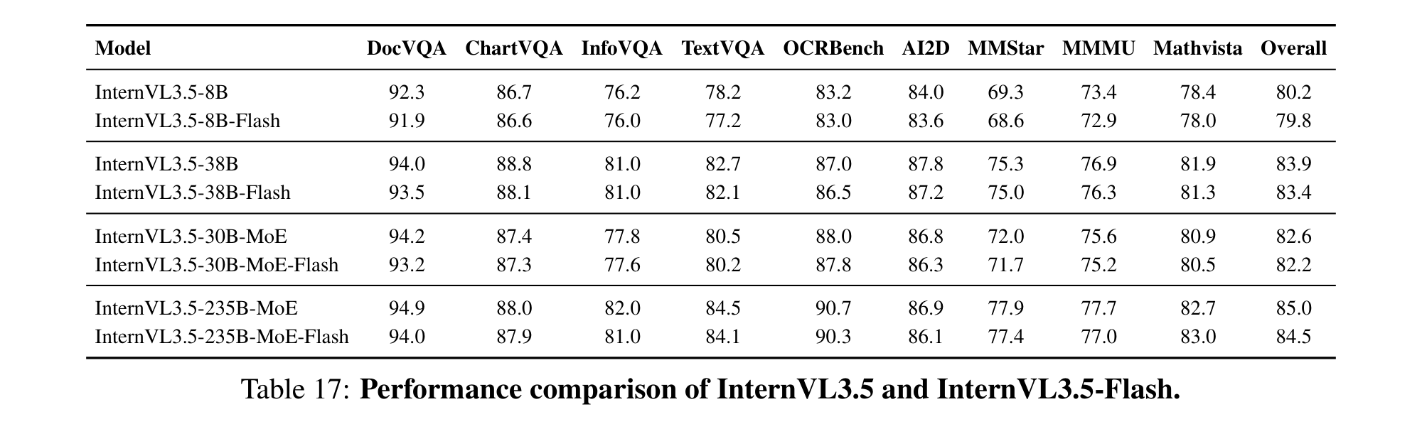
The payoff is that Flash cuts visual tokens by 50% while keeping close to 100% of performance. Table 17's overall scores move from 80.2 → 79.8 (8B), 83.9 → 83.4 (38B), 82.6 → 82.2 (30B MoE) and 85.0 → 84.5 (235B MoE). Combined with DvD, ViR is what turns a ~2x speed-up into the headline 4.05x.
Key Points
- 1
InternVL3.5-Flash = InternVL3.5 + a second pixel shuffle (ξ=161, 64 tokens) + a per-patch router choosing between 64 and 256 tokens
- 2
Dynamic High Resolution adapts to image shape. ViR adds adaptivity to semantic content
- 3
ViCO stage 1, consistency training: the policy at random ξ∈{41,161} matches a frozen reference that always uses ξ=41, via KL
- 4
ViCO stage 2, router training: MLLM frozen, ViR trained as a binary classifier with cross-entropy
- 5
Router labels are self-generated from the loss ratio ri against a dynamic threshold τ (a k-th percentile of a sliding window), which keeps targets balanced
- 6
ViCO uses ~30B tokens. Router data is mainly OCR and VQA, where resolution matters
- 7
Result: ~50% fewer visual tokens with near-identical scores, e.g. 8B overall 80.2 → 79.8, 235B MoE 85.0 → 84.5 (Table 17)
Mathematical Formulation
ViCO Consistency Loss
LViCO=Eξ∼R[N1∑i=1NKL(πθref(yi∣y<i,I)πθpolicy(yi∣y<i,Iξ))]
ξ is drawn uniformly from {41,161}, so Iξ is the image at 256 or 64 tokens per patch. The reference always sees the uncompressed I (equivalently ξ=41). Minimising the KL makes the compressed view reproduce the full view's predictions token by token.
Per-Patch Loss Ratio
ri=LViCO(yi∣I1/4)LViCO(yi∣I1/16)
How much worse the model gets when this patch is squeezed to 64 tokens. A ratio near 1 means compression costs almost nothing.
Router Target
yirouter={0,1,ri<τ(compress: ξ=161)ri≥τ(keep: ξ=41)
τ is the k-th percentile of recent ri values in a sliding window, so it tracks the current loss scale and keeps the two classes balanced.
ViR reduces the work the LLM does on visual tokens. DvD attacks a different cost: the vision encoder and the language model block each other when they share hardware.
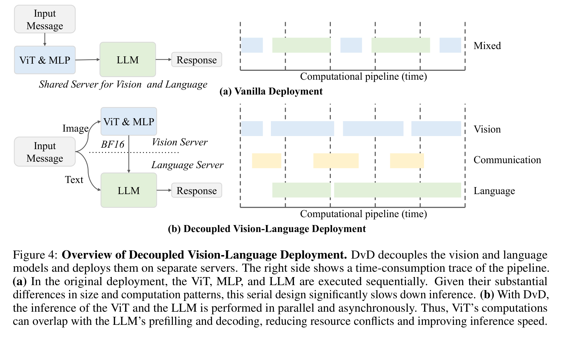
The two halves of an MLLM behave very differently. The ViT is highly parallel and stateless: a batch of image tiles goes in and features come out, with no history. The LLM is autoregressive, needs its KV cache, and is bound by memory bandwidth and latency. In a standard deployment both live on the same GPUs and run serially for each request: ViT, then MLP, then LLM prefill, then decode. While a large ViT (InternViT-6B, say) chews through a high-resolution image, the LLM sits idle, and vice versa.
DvD splits them onto separate servers. The vision server runs the ViT, the MLP and (for Flash) the ViR, batching images and producing compact embeddings. Those are sent one way as BF16 features over TCP, with optional RDMA, to the language server, which runs only the LLM. Vision processing, feature transmission and language processing form an asynchronous three-stage pipeline, so the ViT can work on the next request while the LLM prefills and decodes the current one. Multimodal prefill then behaves close to text-only prefill.
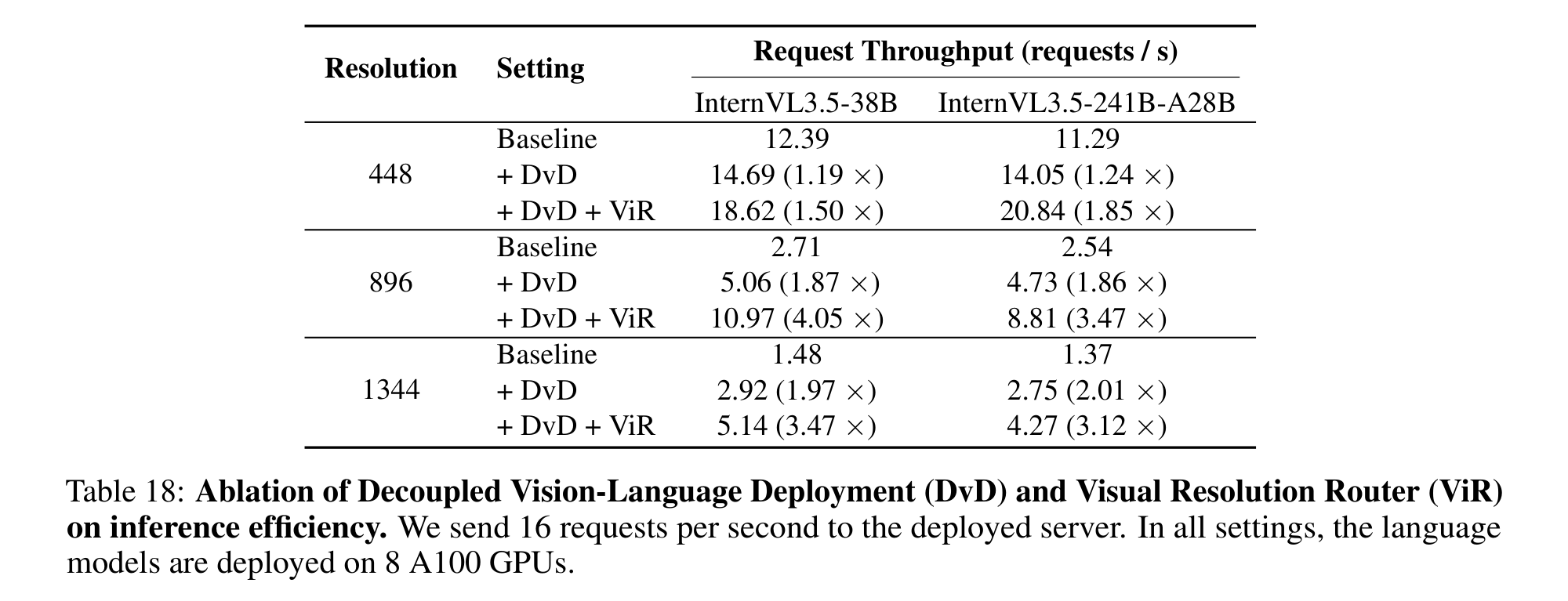
Table 18 measures request throughput at 16 requests per second, with the LLM on 8 A100s. DvD alone gives 1.19x at 448px but 1.97x at 1344px for the 38B model, and 2.01x for 241B-A28B at 1344px. The gain grows with resolution because more tiles mean more vision compute to overlap. Adding ViR on top brings the best case to 4.05x (38B at 896px, 2.71 → 10.97 req/s). The paper expects even larger gains for multi-image and video input, where patch counts grow further. A secondary benefit is operational: vision and language hardware can be sized and upgraded independently, and new vision modules can be added without touching the language server.
Key Points
- 1
The ViT is parallel and stateless. The LLM is autoregressive and memory-bound. On shared GPUs each blocks the other
- 2
DvD places ViT + MLP (+ ViR) on a vision server and only the LLM on a language server
- 3
Communication is one-way BF16 features over TCP, optionally RDMA
- 4
Vision, transfer and language form an asynchronous three-stage pipeline, so ViT work overlaps LLM prefill and decode
- 5
Table 18, 38B: DvD gives 1.19x at 448px, 1.87x at 896px and 1.97x at 1344px. The speed-up grows with resolution
- 6
DvD + ViR: up to 4.05x (38B, 896px: 2.71 → 10.97 req/s) and 3.47x for 241B-A28B at the same resolution
- 7
Hardware for each side can be scaled independently, and new vision modules don't require redeploying the language server
Mathematical Formulation
Why Overlap Helps
Tserial≈∑k(tvis(k)+tllm(k))⟶TDvD≈∑kmax(tvis(k),tllm(k))
A simplified pipeline view (not an equation from the paper) for a stream of requests k. Once vision and language run concurrently on separate hardware, steady-state cost per request approaches the slower of the two stages rather than their sum. The larger tvis is (bigger ViT, more tiles), the more there is to hide, which matches the resolution trend in Table 18.
On top of training, InternVL3.5 can spend extra compute at inference on reasoning problems. The paper scales along two axes.
Deep thinking increases reasoning depth. With Thinking mode switched on, the model breaks a problem into logical steps and checks intermediate conclusions before it commits to an answer. The SFT stage instils this behaviour using the filtered Thinking-mode traces.
Parallel thinking increases breadth. Following InternVL3, the model samples several candidate solutions and VisualPRM-v1.1, a multimodal process reward model, picks the best one (Best-of-N). Because a process reward model scores each step rather than only the final answer, it can prefer a sound derivation over one that reached the right number by luck.
Two caveats are easy to miss. Unless stated otherwise, every headline number in the paper is reported without test-time scaling. And TTS was applied only to reasoning benchmarks: the authors report that perception and understanding tasks gain nothing significant from it.
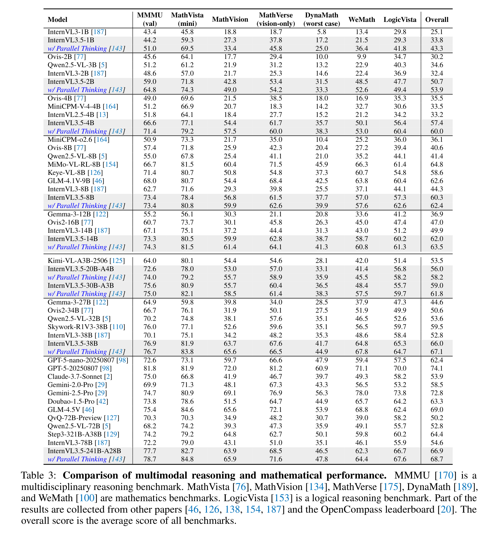
When it is used, TTS stacks on top of Cascade RL. Parallel thinking lifts the overall reasoning score (Table 3) of InternVL3.5-4B from 57.4 → 60.0, 8B from 60.3 → 62.4, and 241B-A28B from 66.9 → 68.7. The gains are largest at small scale: the 1B model jumps from 33.8 → 43.3.
Key Points
- 1
Deep thinking: Thinking mode produces step-by-step reasoning with intermediate validation and adds depth
- 2
Parallel thinking: Best-of-N with VisualPRM-v1.1 as the critic adds breadth
- 3
Headline results in the paper are reported without TTS unless noted
- 4
TTS is applied only to reasoning benchmarks. Perception tasks showed no significant gain
- 5
Gains stack with Cascade RL: +2.6 (4B), +2.1 (8B), +1.8 (241B-A28B) points on overall reasoning
- 6
Small models benefit most: InternVL3.5-1B goes from 33.8 → 43.3 with parallel thinking (Table 3)
Mathematical Formulation
Best-of-N with a Process Reward Model
y^=argmaxy∈{y1,…,yN}PRM(x,y),yj∼πθ(⋅∣x)
Sample N reasoning chains, have VisualPRM score each one (aggregating its per-step scores) and return the highest-scoring chain. Compute grows linearly with N, and none of it is spent on training.
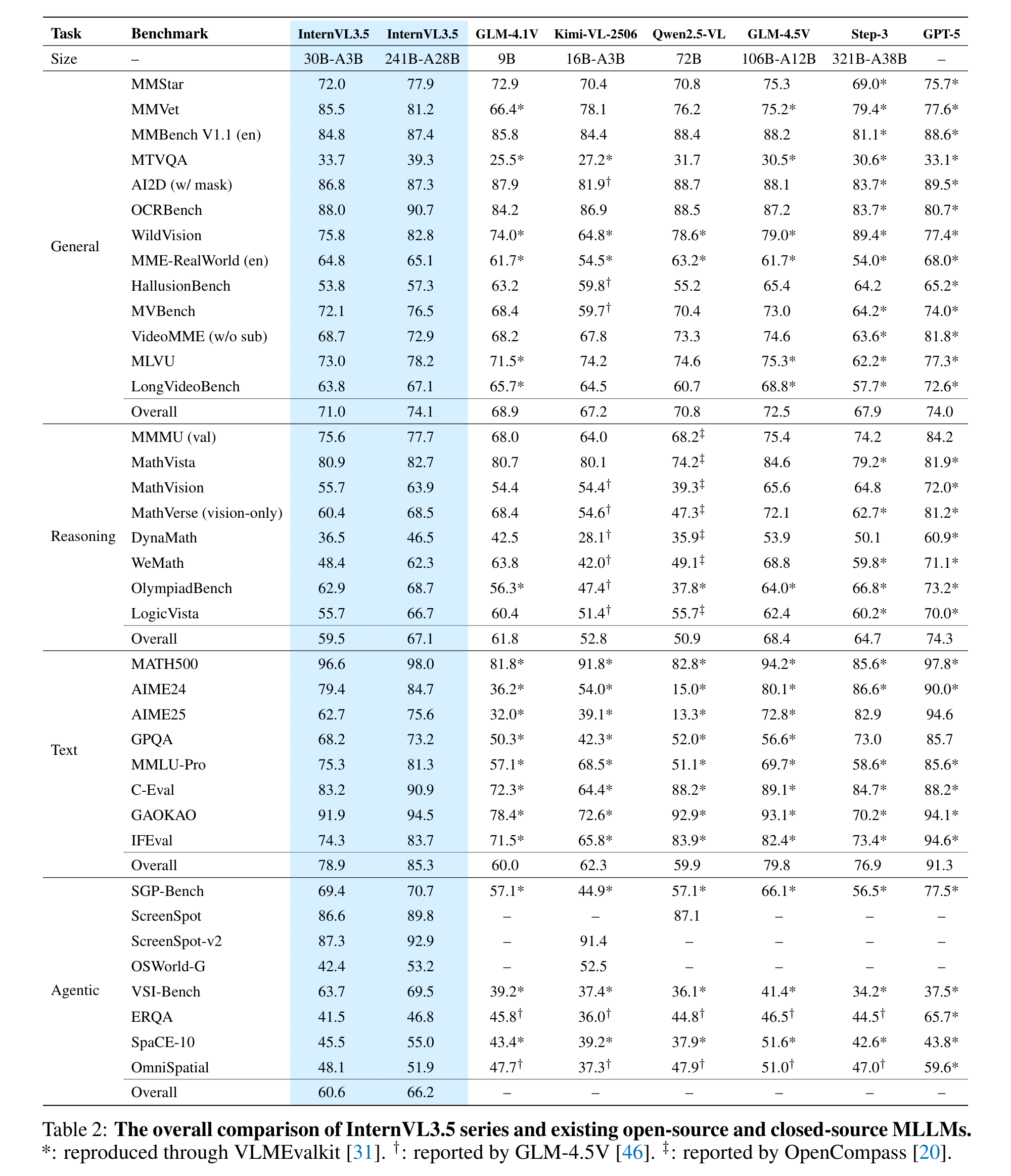
Table 2 compares the two flagship models with the strongest open MLLMs and GPT-5 across 35 benchmarks in four groups. InternVL3.5-241B-A28B scores 74.1 overall on general multimodal tasks against GPT-5's 74.0, leads open-source models on MMVet, MTVQA, OCRBench and MME-RealWorld, and scores 77.7 on MMMU and 82.7 on MathVista. On text it scores 85.3 overall (GLM-4.5V 79.8, Step-3 76.9, GPT-5 91.3), including 84.7 on AIME24 and 81.3 on MMLU-Pro.
Most of the reasoning gain comes from Cascade RL, and Table 15 (plotted in Figure 5) breaks it down by stage. At 2B, InternVL3 averages 32.4 on the reasoning suite. InternVL3.5 after SFT reaches 38.5, after MPO 41.1, and after the full Cascade RL 50.7, which is +12.2 points over its own SFT model. At 241B-A28B the progression is 60.4 → 62.4 → 66.9 (+6.5), against InternVL3-78B's 54.6. The gain is consistent across every size and both dense and MoE models. The smaller the model, the larger the relative lift.
Mid-size models hold up well. On MMMU, InternVL3.5-30B-A3B (75.6) and 14B (73.3) both beat the much larger InternVL3-78B (72.2). Text ability survives multimodal training intact: InternVL3.5-1B beats its own Qwen3-0.6B initialisation on 15 of 16 text benchmarks (+6.7 overall), and the 241B model gains +2.3 over Qwen3-235B-A22B.
Some weaknesses remain, and the paper says so. HallusionBench is the clearest: 57.3 for 241B-A28B versus 65.4 for GLM-4.5V and 65.2 for GPT-5. Reasoning still trails GPT-5 by a wide margin (67.1 vs 74.3 in Table 2's reasoning group). One reading note: the reasoning "overall" for 241B-A28B is 66.9 in Table 3 but 67.1 in Table 2, because the two tables average different benchmark sets (Table 2 adds OlympiadBench).
Key Points
- 1
General multimodal overall: 74.1 for InternVL3.5-241B-A28B vs 74.0 for GPT-5 (Table 2)
- 2
Reasoning: 77.7 MMMU, 82.7 MathVista, overall 67.1 (GPT-5 74.3, GLM-4.5V 68.4)
- 3
Text overall 85.3, ahead of every open MLLM in Table 2 (GPT-5 91.3)
- 4
Cascade RL lifts the reasoning average at every size, e.g. 2B 38.5 → 50.7 (+12.2) and 241B-A28B 60.4 → 66.9 (+6.5) over SFT (Table 15)
- 5
InternVL3.5-8B after SFT alone already beats InternVL3-8B by +9.3 (53.6 vs 44.3)
- 6
Mid-size MMMU: 30B-A3B 75.6 and 14B 73.3 both beat InternVL3-78B (72.2)
- 7
Language preserved: 1B beats Qwen3-0.6B on 15/16 text benchmarks (+6.7). 241B gains +2.3 over Qwen3-235B-A22B (Table 14)
- 8
Weak spot: HallusionBench 57.3 vs 65.4 (GLM-4.5V) and 65.2 (GPT-5)
Mathematical Formulation
Where the Reasoning Gain Comes From (241B-A28B)
InternVL3-78B54.6SFTInstruct60.4MPOMPO62.4GSPOCascade RL66.9
The averages over seven reasoning benchmarks in Table 15. Better data and SFT account for the first jump. Of the remaining 6.5 points from Cascade RL, the online GSPO stage contributes most, building on the MPO warm-up.
The "versatility" in the title refers to capabilities that InternVL3 largely lacked, added through the capability-expansion SFT data and then sharpened by RL.
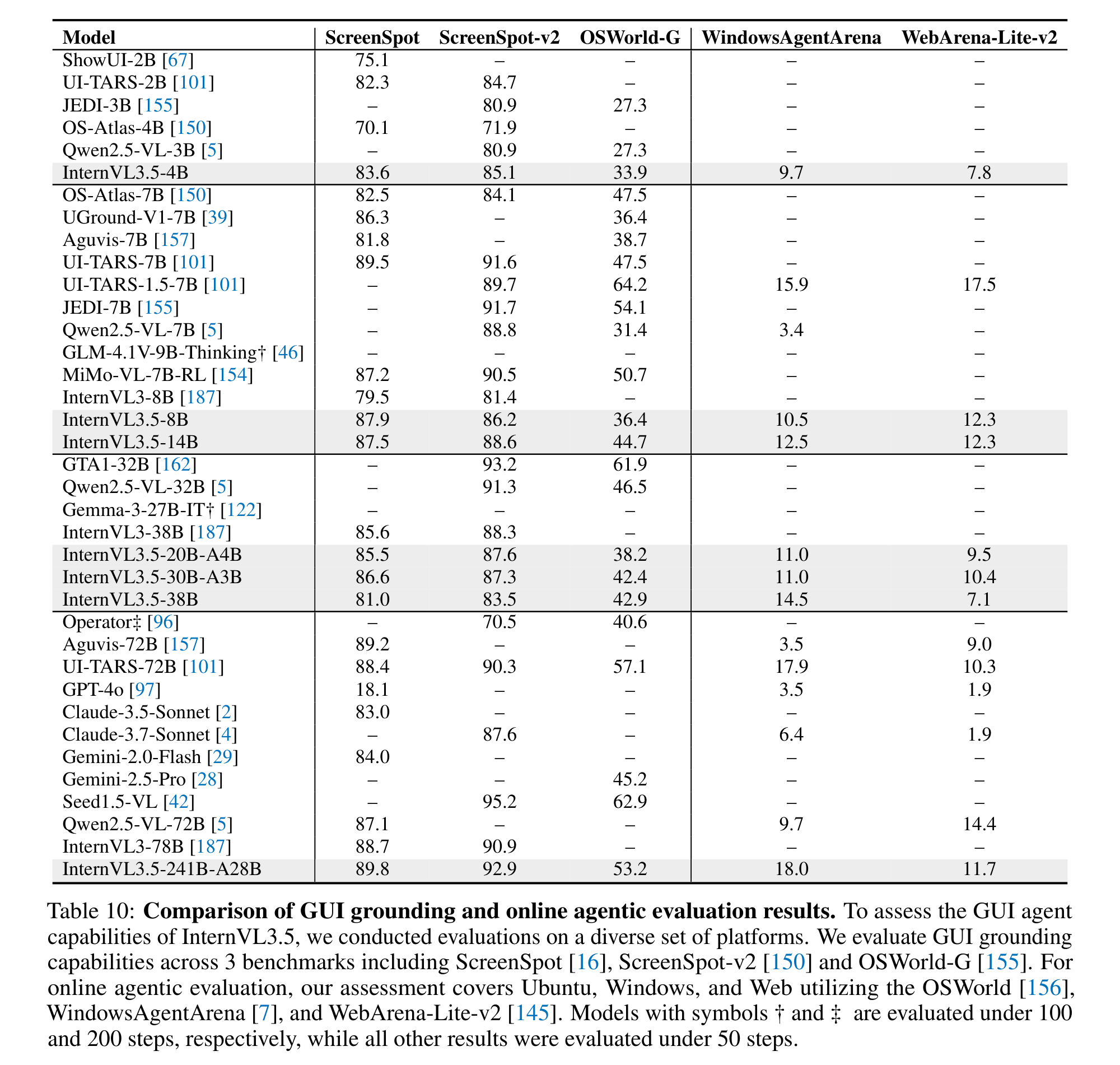
GUI agents (Table 10). On GUI grounding, InternVL3.5-241B-A28B scores 92.9 on ScreenSpot-v2, which is +2.6 over the specialist UI-TARS-72B and close to the commercial Seed1.5-VL's 95.2. It reaches 53.2 on OSWorld-G. In online agent environments it scores 18.0 on WindowsAgentArena, +8.3 over Qwen2.5-VL-72B, while GPT-4o manages 3.5. On WebArena-Lite-v2 it scores 11.7 to GPT-4o's 1.9. The absolute numbers are still low, which shows how hard real computer-use tasks remain, but InternVL3.5 is the strongest generalist MLLM in the table.
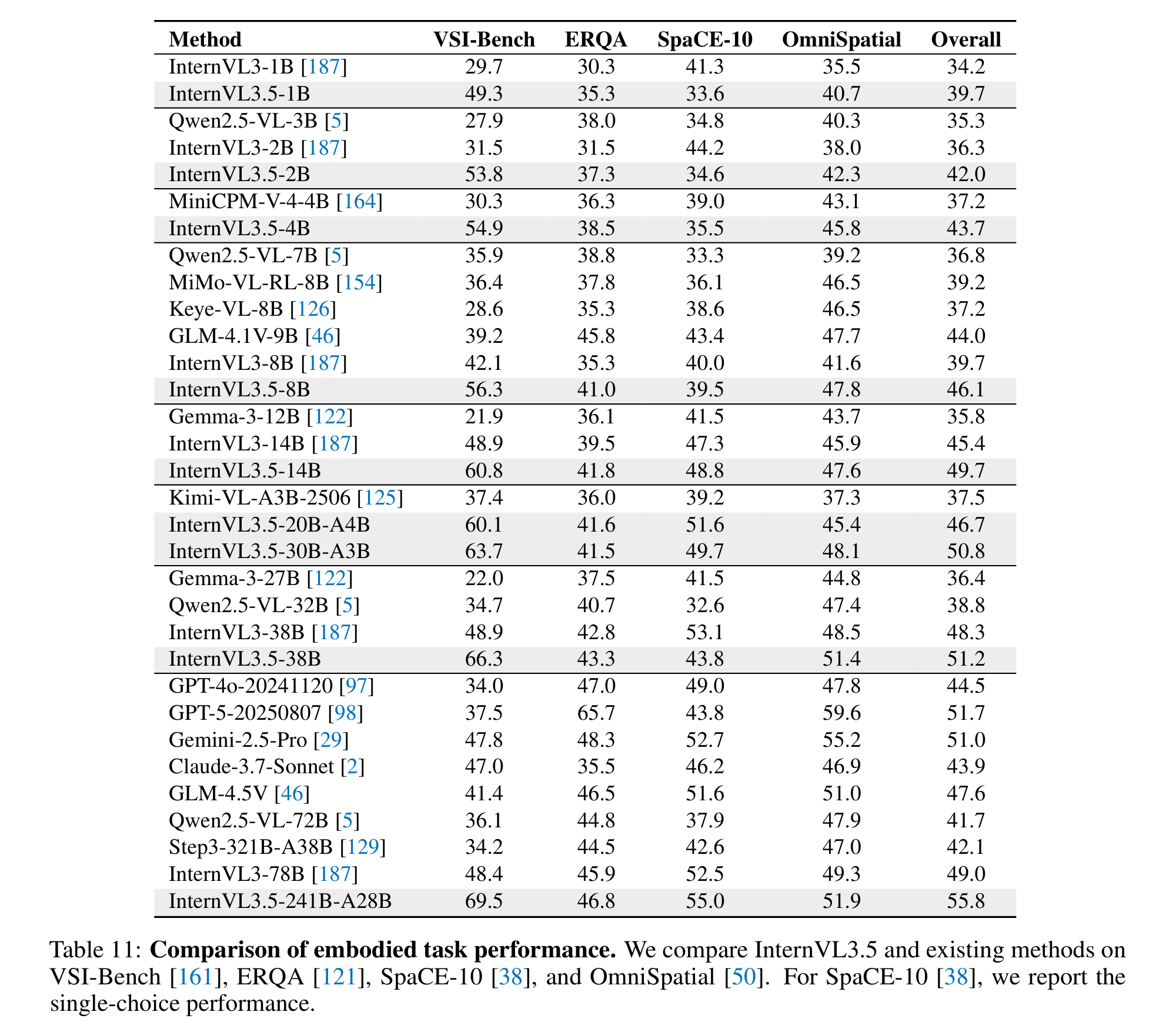
Embodied and spatial reasoning (Table 11). On VSI-Bench, the most widely used spatial benchmark, even InternVL3.5-1B scores 49.3, +19.6 over InternVL3-1B and ahead of Qwen2.5-VL-72B's 36.1. Scaling to 241B-A28B reaches 69.5. On ERQA the flagship scores 46.8, near Gemini-2.5-Pro's 48.3, and it posts the highest overall score in the table (55.8).
SVG understanding and generation. On SGP-Bench, which asks questions about images given only their SVG code, 241B-A28B reaches 70.7, a new open-source best but still behind GPT-5's 77.5. On SArena-Icon Text2SVG it reaches an FID of 11.27, and the 38B model's 14.56 beats GPT-4o's 15.18.
The broader point is that one set of open weights now covers GUI operation, spatial reasoning and code-as-graphics, alongside the usual VQA and OCR, at quality within reach of commercial systems.
Key Points
- 1
ScreenSpot-v2 92.9 for 241B-A28B: +2.6 over UI-TARS-72B and close to Seed1.5-VL (95.2)
- 2
Online agents: WindowsAgentArena 18.0 (+8.3 over Qwen2.5-VL-72B, GPT-4o 3.5) and WebArena-Lite-v2 11.7 (GPT-4o 1.9)
- 3
VSI-Bench: 1B scores 49.3 (+19.6 over InternVL3-1B) and 241B-A28B scores 69.5
- 4
ERQA 46.8 vs Gemini-2.5-Pro 48.3. Highest embodied overall in Table 11 (55.8)
- 5
SGP-Bench 70.7 (best open model) vs GPT-5 77.5
- 6
Text2SVG FID 11.27 (241B). The 38B's 14.56 beats GPT-4o's 15.18
- 7
These skills come from the SFT capability-expansion data (GUI, embodied, SVG), not from architecture changes
Keep reading
Related Papers
Go deeper