Qwen2.5
18T-Token Pre-training, Hyper-parameter Scaling Laws, and SFT + DPO + GRPO Post-training for an Open 0.5B–72B LLM Family
Qwen Team
10
Concepts
12
Formulas
8
Figures
5
Demos
Paper Overview
Qwen2.5 (Qwen Team, Alibaba — arXiv 2412.15115, Dec 2024) has an unusual thesis for a technical report: the architecture is nearly the same as last time, and that is intentional. Qwen2.5 keeps Qwen2's dense decoder — GQA, SwiGLU, RoPE, QKV bias, RMSNorm — and puts its effort into the parts of the pipeline other than the architecture.
On the pre-training side, the dataset grows from 7T to 18T tokens, built by previous-generation Qwen models that score, synthesise and rebalance web data. Scaling laws are used to predict optimal learning rate and batch size, not only model size, across nine production models. Context is extended in stages, with RoPE base changes and training-free YaRN + Dual Chunk Attention at inference.
On the post-training side, over 1M SFT examples are filtered by verifiers, then RL runs in two stages. Offline DPO handles domains where answers can be checked mechanically, and online GRPO with a learned reward model handles helpfulness, truthfulness and harmlessness.
The open release spans 0.5B to 72B (base and instruct, plus quantized variants), alongside two API-only MoE models, Qwen2.5-Turbo (1M-token context) and Qwen2.5-Plus. The flagship Qwen2.5-72B-Instruct beats Llama-3.1-405B-Instruct on MATH (83.1 vs 73.8), LiveCodeBench (55.5 vs 41.6) and Arena-Hard (81.2 vs 69.3) at about a fifth of its size. Qwen2.5 also became the base for Qwen2.5-Math, Qwen2.5-Coder, QwQ and Qwen2.5-VL.
Chapter Roadmap
Click any topic to jump in
7T → 18T Tokens
Qwen2-scored filtering, Math/Coder corpora, reward-filtered synthetic data and domain rebalancing make 18T tokens worth training on.
Architecture and tuning
Model Family
Seven dense sizes from 0.5B to 72B with GQA, SwiGLU, RoPE and QKV bias, plus API-only MoE models Turbo and Plus.
Hyper-parameter Scaling Laws
Optimal learning rate and batch size predicted from model size and data size, fitted on 44M–14B runs.
Long-Context Pre-training
4K → 32K with RoPE base 10^6; Turbo climbs to 262K; YaRN + DCA add 4x at inference.
Supervised Fine-tuning
Over 1M verified examples across nine skill areas, with outputs up to 8K tokens.
Two-stage RL
Offline RL (DPO)
~150K pass/fail pairs graded by execution and answer matching, where reward models struggle.
Online RL (GRPO)
A six-criterion reward model, 8 samples per query, and high-variance queries trained first.
Signals and scale
Reward Model Evaluation
No RM wins every benchmark, and RM scores fail to predict the quality of the RL policy.
1M-Token Context
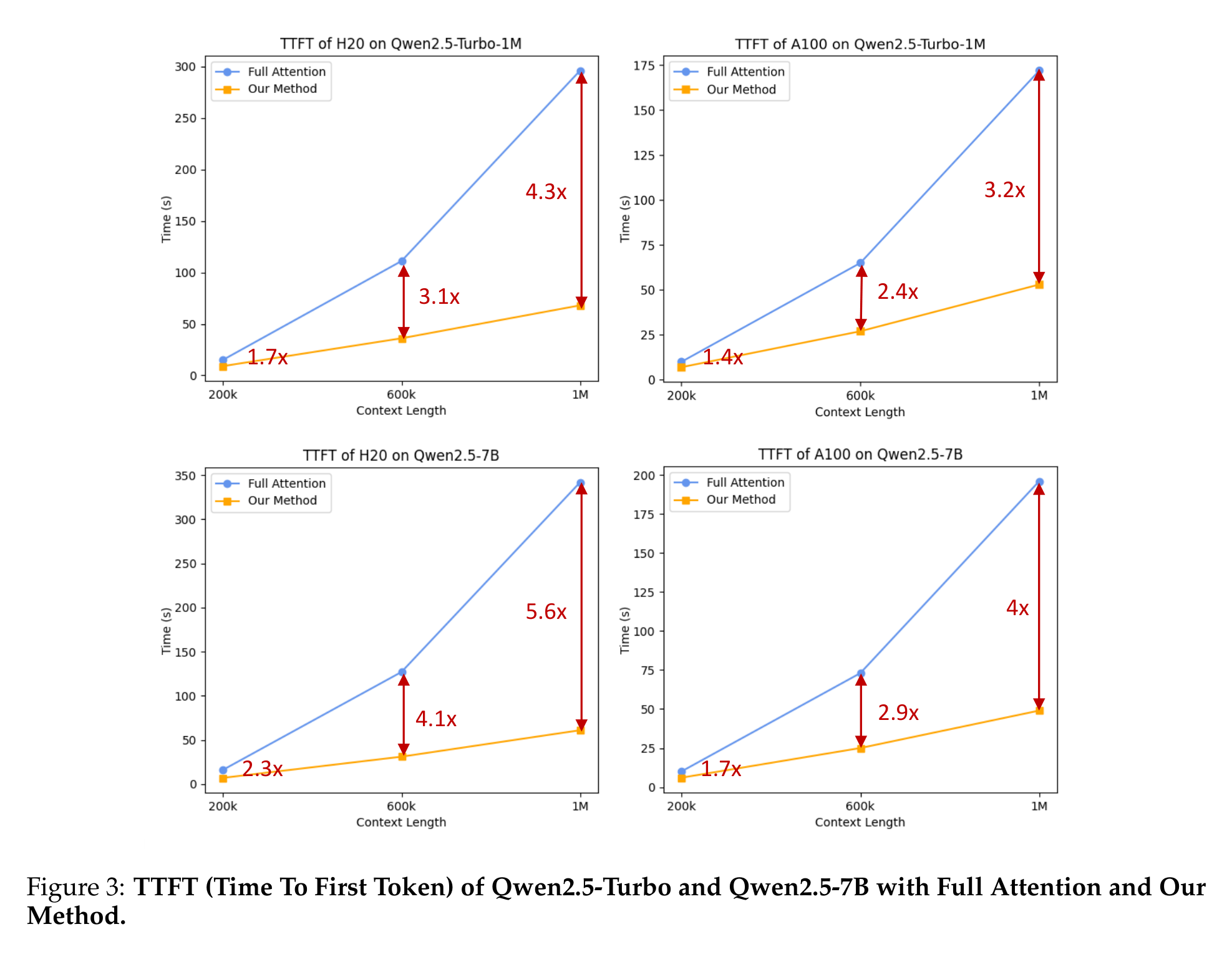
Two-stage long SFT, short-only RL, 100% passkey at 1M, and 3.2–4.3x faster TTFT via sparse attention.
Results
72B-Instruct beats Llama-3.1-405B-Instruct on 7 of 13 instruct benchmarks at about 1/5.6 of its size.
Concept by concept
10 sections, in reading order.
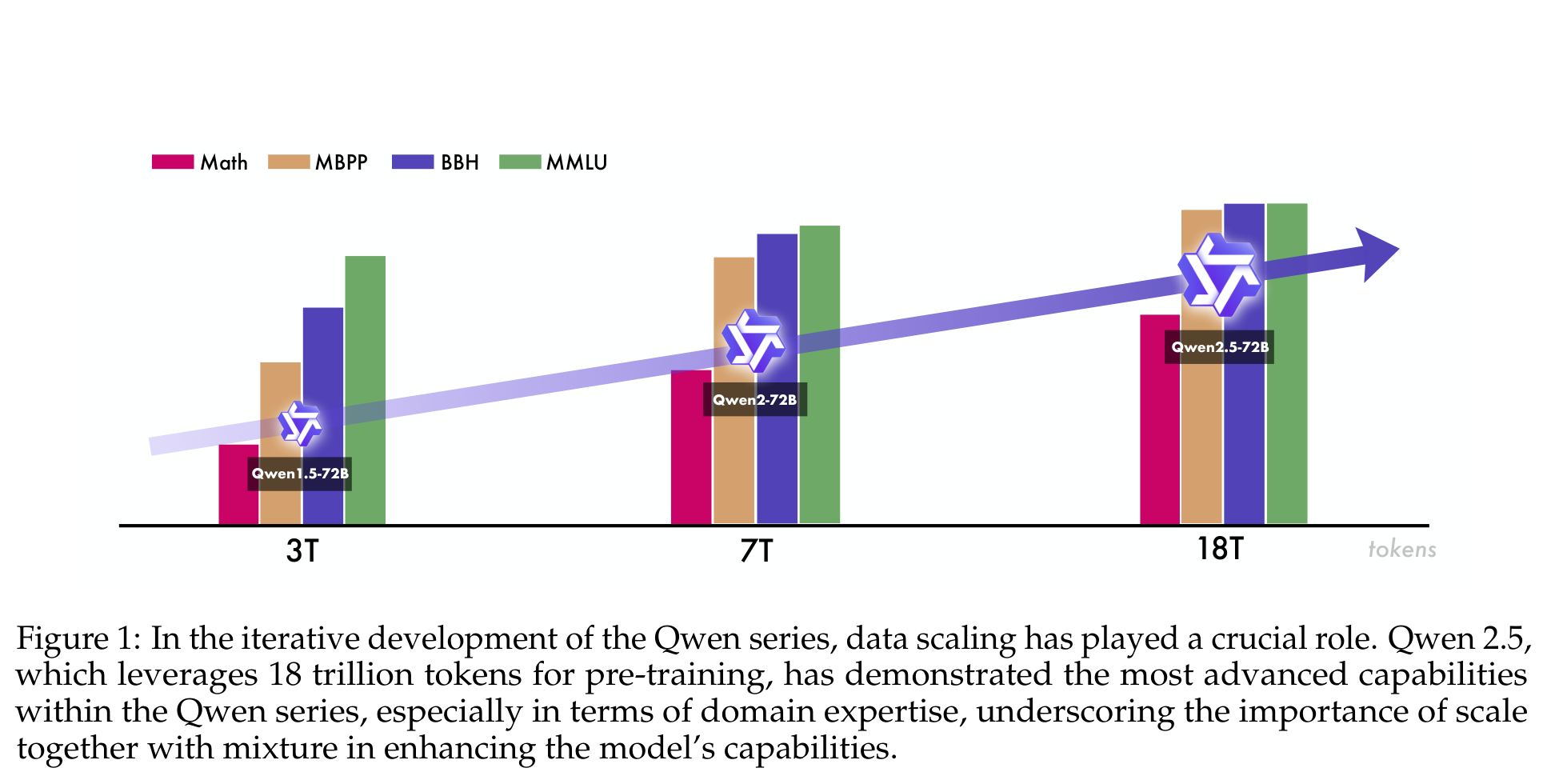
Qwen2.5 keeps Qwen2's architecture almost untouched. What changes is the data, and the report is blunt about where it thinks capability comes from: Figure 1 plots the Qwen series against pre-training tokens — 3T for Qwen1.5, 7T for Qwen2, 18T for Qwen2.5 — and credits "scale together with mixture" for the gains.
Scale alone would be easy to describe and hard to make useful. Web-scale crawls are dominated by whatever the internet produces most of, and the paper names it: e-commerce, social media and entertainment are heavily over-represented, often as repetitive, template-based or machine-generated text, while technology, science and academic research — the domains that carry dense information — are under-represented. Simply collecting 2.5x more of the same distribution would mostly buy 2.5x more product listings.
So the 18T tokens are the output of four interventions. Filtering: Qwen2-Instruct models score every sample along multiple dimensions, which works better than Qwen2's filter because Qwen2 itself was trained on a larger multilingual corpus. Domain data: the math and code corpora built for Qwen2.5-Math and Qwen2.5-Coder are folded directly into general pre-training. Synthetic data: Qwen2-72B-Instruct and Qwen2-Math-72B-Instruct generate math, code and knowledge text, which is then filtered by a general reward model and by Qwen2-Math-RM-72B. Mixture: Qwen2-Instruct classifies content by domain, over-represented domains are down-sampled and high-value domains up-sampled.
The pattern worth noticing is self-bootstrapping. Every one of the four steps uses a previous-generation Qwen model as a judge, a generator or a classifier. The model family is now a component of its own data pipeline — the same move that lets later models in the series (QwQ, Qwen2.5-Math, Qwen2.5-VL) build on Qwen2.5 in turn.
Key Points
- 1
Pre-training data grows from 7 trillion tokens (Qwen2) to 18 trillion tokens (Qwen2.5), with a focus on knowledge, coding and mathematics
- 2
Better filtering: Qwen2-Instruct models act as multi-dimensional quality scorers — improving both retention of good data and removal of bad data across languages
- 3
Better math and code: training data from Qwen2.5-Math and Qwen2.5-Coder is integrated directly into general pre-training
- 4
Better synthetic data: generated by Qwen2-72B-Instruct and Qwen2-Math-72B-Instruct, then filtered by a proprietary general reward model and Qwen2-Math-RM-72B
- 5
Better mixture: e-commerce, social media and entertainment are down-sampled; technology, science and academic research are up-sampled
- 6
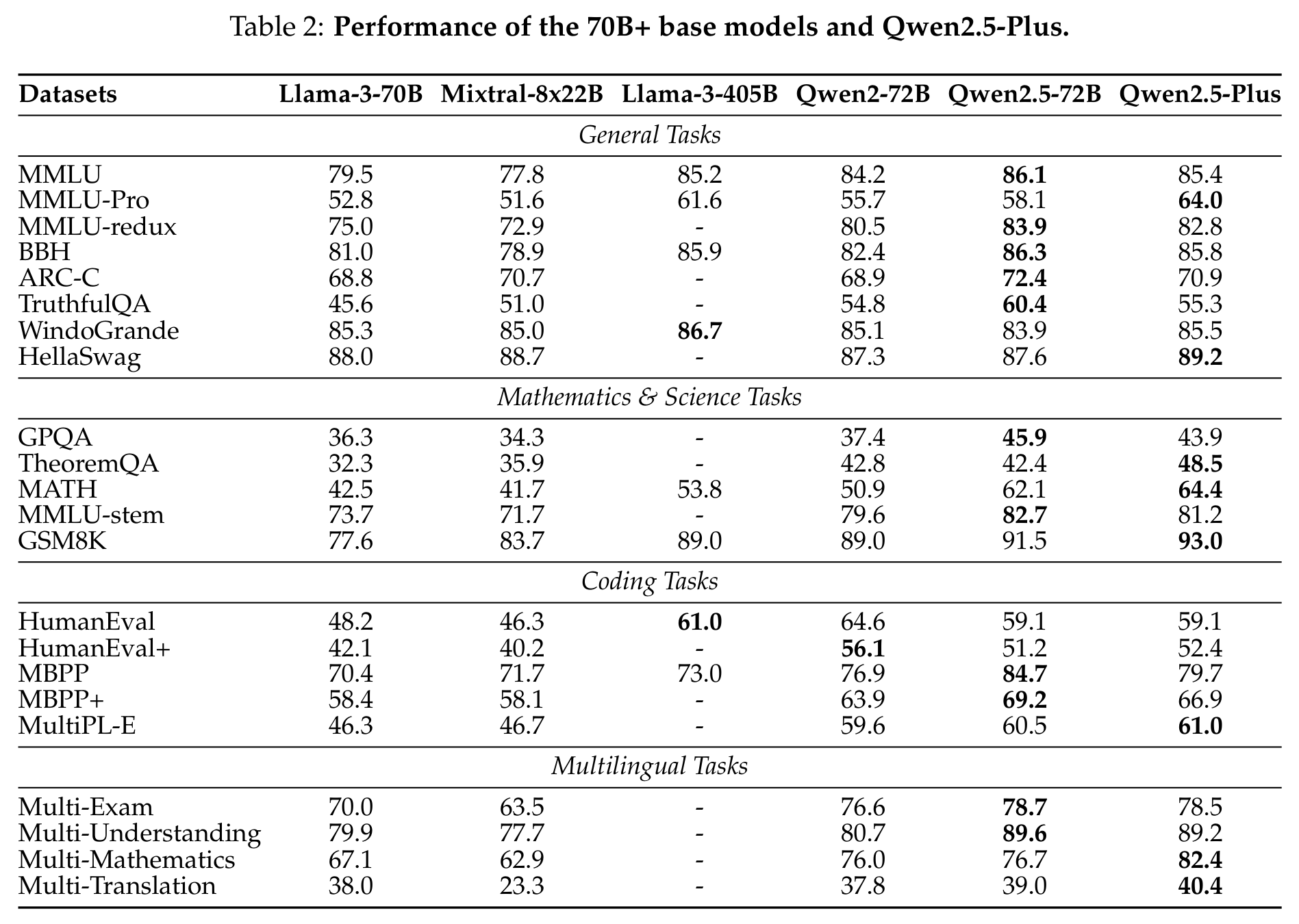
On base models the effect is visible in Table 2: Qwen2-72B → Qwen2.5-72B moves MMLU 84.2 → 86.1, MATH 50.9 → 62.1, MBPP 76.9 → 84.7
The open-weight release is seven dense decoder-only models — 0.5B, 1.5B, 3B, 7B, 14B, 32B and 72B — each as a base and an instruction-tuned model, plus quantized variants; over 100 checkpoints in total. Qwen2 had skipped 3B, 14B and 32B. Qwen2.5 brings them back on the argument that these middle sizes are the most cost-effective for resource-limited deployments and are under-served by other open families.
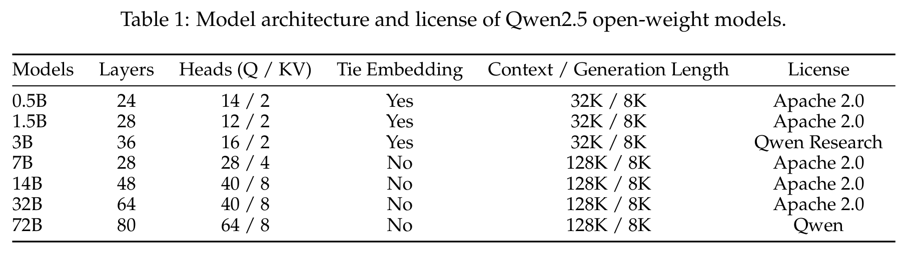
The architecture is deliberately conservative and identical to Qwen2: a pre-norm Transformer decoder with RMSNorm, SwiGLU feed-forward layers, RoPE positions, QKV bias in attention, and Grouped Query Attention. Table 1 shows the GQA ratios. The 72B model has 64 query heads but only 8 key-value heads, so each KV head is shared by 8 query heads and the KV cache is 8x smaller than full multi-head attention would need. The three smallest models also tie input and output embeddings, which matters when a 151K-token vocabulary is a large fraction of a 0.5B model.
Two proprietary models, Qwen2.5-Turbo and Qwen2.5-Plus, are Mixture-of-Experts variants served via API. They replace each FFN with an MoE layer that routes every token to its top-K experts, using the fine-grained expert segmentation and shared-expert routing of Qwen1.5-MoE and DeepSeekMoE: many small experts rather than a few large ones, plus experts every token always passes through. The report does not publish their expert counts or parameter sizes; it says only that hyper-parameters were tuned so they match specific dense models — Plus is positioned against Qwen2.5-72B, Turbo against Qwen2.5-14B.
The tokenizer is unchanged in substance — byte-level BPE with 151,643 regular tokens — but the control-token set grows from 3 to 22, including two new tokens for tool use. Every Qwen2.5 model shares this vocabulary, so tool-calling formats and chat templates transfer across the whole family.
Key Points
- 1
Dense open-weight sizes: 0.5B / 1.5B / 3B / 7B / 14B / 32B / 72B — 3B, 14B and 32B return after being absent from Qwen2
- 2
Architecture: Transformer decoder with GQA, SwiGLU, RoPE, QKV bias and pre-norm RMSNorm — unchanged from Qwen2
- 3
GQA ratios from Table 1: 72B uses 64 / 8 heads (8 query heads per KV head); 7B uses 28 / 4; 0.5B uses 14 / 2
- 4
0.5B, 1.5B and 3B tie input and output embeddings; context is 32K for those three and 128K for 7B and above, with an 8K generation length throughout
- 5
Licenses: Apache 2.0 for most sizes; 3B uses the Qwen Research license and 72B the Qwen license
- 6
Qwen2.5-Turbo and Qwen2.5-Plus are API-only MoE models with fine-grained experts and shared-expert routing
- 7
Tokenizer: byte-level BPE, 151,643 regular tokens, control tokens expanded from 3 to 22 (two reserved for tools)
Mathematical Formulation
GQA Key-Value Sharing
g=nkvnq,KV cacheMHAKV cacheGQA=nqnkv=g1
Each of the nkv key-value heads serves a group of g query heads. For Qwen2.5-72B, nq=64 and nkv=8, so g=8 and the cache that dominates long-context inference memory is one eighth of the multi-head size.
MoE Layer with Shared Experts
y=∑j∈SEj(x)+∑i∈TopK(g(x))gi(x)Ei(x)
The generic form of the shared-expert design the report adopts from Qwen1.5-MoE and DeepSeekMoE: experts in S process every token, while the router g sends each token to its top-K routed experts. The report does not disclose K or the expert counts for Turbo and Plus.
Scaling laws are usually used to answer one question: given a compute budget, how big should the model be and how many tokens should it see? Chinchilla and Llama 3 use them that way. Qwen2.5 turns them toward a more operational question: given a model of size N trained on D tokens, what learning rate and batch size should it use?
This matters because Qwen2.5 trains nine production models — seven dense sizes and two MoE variants — and tuning the learning rate μ and batch size B by trial at 72B scale is not affordable. Instead the team ran a sweep of small and medium runs, dense models from 44M to 14B parameters and MoE models from 44M to 1B activated parameters, on 0.8B to 600B tokens, found the optimal μopt and Bopt at each point, and fit how those optima move with N and D. The fit is then extrapolated to the production sizes.
With optimal hyper-parameters predicted, the same data supports a second fit: final loss as a function of architecture and data scale. That is what makes the MoE design tractable. The team uses it to predict how MoE models with various total and activated parameter counts compare with dense models, and picks configurations that land at parity with specific dense models such as Qwen2.5-72B and Qwen2.5-14B — the positioning of Plus and Turbo.
One caveat is worth stating plainly: the report describes this methodology but publishes no fitted coefficients, exponents or curves. Readers can reproduce the approach, but not check the numbers.
Key Points
- 1
Scaling laws are used to choose hyper-parameters — learning rate μ and batch size B — rather than only model size
- 2
The sweep covers dense models from 44M to 14B parameters and MoE models from 44M to 1B activated parameters, on 0.8B to 600B tokens
- 3
Optimal μopt and Bopt are modelled as functions of model size N and data size D
- 4
With those optima fixed, final loss is modelled against architecture and data scale
- 5
The loss model predicts MoE vs dense performance, so MoE activated and total parameters can be tuned to match Qwen2.5-72B and Qwen2.5-14B
- 6
The report gives no fitted coefficients — the method is described, not the curves
Mathematical Formulation
What the Hyper-parameter Laws Predict
μopt=fμ(N,D),Bopt=fB(N,D)
The optimal learning rate and batch size are fitted as functions of non-embedding model size N and training tokens D across the 44M–14B sweep, then extrapolated. The paper does not publish the functional form of fμ or fB.
The Chinchilla-style Loss Model it Builds On
L(N,D)=E+NαA+DβB′
The parametric loss form of Hoffmann et al. (2022), which the report cites as a starting point. Qwen2.5 fits final loss as a function of architecture and data scale under predicted optimal hyper-parameters; its own fitted constants are not reported. B′ is a fitted constant, unrelated to batch size B.
Training on long sequences from the start is wasteful: attention cost grows with sequence length and most pre-training knowledge does not need 32K tokens of context. Qwen2.5 therefore pre-trains in two phases. The bulk of training runs at 4,096 tokens; the final stage extends every model except Turbo to 32,768 tokens.
Extending context is mostly a positional-encoding problem. RoPE rotates query and key pairs at frequencies θi=b−2i/d; with the default base b=10,000 the slowest dimensions complete their rotation well before 32K tokens, so distant positions alias with nearby ones. Qwen2.5 applies ABF (adjusted base frequency) and raises the base from 10,000 to 1,000,000 during the extension stage. A larger base stretches every wavelength, so the model sees distinct rotations across the longer window.
Qwen2.5-Turbo targets 1M tokens and goes further with a progressive four-stage schedule: 32,768 → 65,536 → 131,072 → 262,144 tokens, with RoPE base 10,000,000. At each stage the data is 40% sequences at the current maximum length and 60% shorter sequences, so the model adapts to longer inputs without losing its behaviour on short ones.
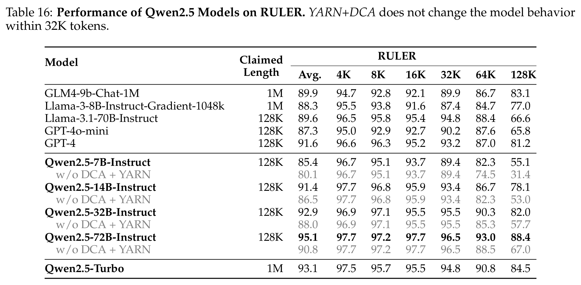
Training stops at 32K (or 262K for Turbo), but inference goes further. YaRN rescales RoPE frequencies at inference time, and Dual Chunk Attention (DCA) splits a long sequence into chunks and remaps relative positions so no query–key distance exceeds what was seen in training. Together they give a four-fold increase: open models reach 131,072 tokens and Turbo reaches 1 million. Both are training-free and leave behaviour within 32K unchanged, which is why the RULER table's "w/o DCA + YARN" rows match the full rows up to 32K and diverge only beyond it.
Key Points
- 1
Two-phase pre-training: most training at 4,096 tokens, then a final stage at 32,768 tokens for all models except Turbo
- 2
RoPE base frequency raised from 10,000 to 1,000,000 via ABF during context extension
- 3
Qwen2.5-Turbo: progressive stages 32,768 → 65,536 → 131,072 → 262,144 tokens with RoPE base 10,000,000
- 4
Each Turbo stage mixes 40% sequences at the current maximum length with 60% shorter sequences
- 5
YaRN + Dual Chunk Attention at inference give a 4x length increase: 131,072 tokens for open models and 1M for Turbo
- 6
Both techniques are training-free and do not change model behaviour within 32K tokens
Mathematical Formulation
RoPE Frequencies and the ABF Base Change
θi=b−2i/d,λi=θi2π=2πb2i/d,b:104→106
Dimension pair i rotates at frequency θi with wavelength λi. Raising the base b stretches every wavelength, so the slow dimensions keep distinguishing positions across a 32K window. Qwen2.5-Turbo uses b=107.
Inference-time Extension
Linfer≈4×Ltrain:32,768→131,072,262,144→1,048,576
YaRN and DCA together give the four-fold increase the report claims: the open-weight models trained at 32K serve 128K, and Turbo trained at 256K serves about 1M tokens.
Post-training in Qwen2.5 is a three-step pipeline — SFT, then offline RL, then online RL — and SFT carries most of the data. The team built over 1 million SFT examples, organised around the specific places Qwen2 fell short.
The most user-visible gap was length. Typical post-training responses stay under about 2,000 tokens, so models learn to stop early. Qwen2.5 targets 8,192-token outputs by building long-response data: it back-translates long pre-training documents into the queries that would have produced them, imposes output-length constraints, and filters weak pairs with Qwen2.
The remaining areas share one idea: verify before you train. Math uses Qwen2.5-Math chain-of-thought data with rejection sampling guided by a reward model and reference answers. Code uses Qwen2.5-Coder's multi-agent instruction data across nearly 40 programming languages, checked in a multilingual sandbox with static analysis and unit tests. Instruction-following data is generated together with verification code and unit tests, and kept only if execution feedback confirms compliance. Logical reasoning adds 70,000 new queries; structured-data understanding adds tables and semi-structured inputs with reasoning chains; cross-lingual data is translated and then checked for semantic alignment; and hundreds of system prompts make the model robust to how it is instructed. A final response filter keeps only outputs judged flawless by both a critic model and a multi-agent scoring system.
Training is short and conservative: two epochs at 32,768-token sequences, learning rate decayed from 7×10⁻⁶ to 7×10⁻⁷, weight decay 0.1, gradient clipping at 1.0.
Key Points
- 1
Over 1 million SFT examples covering nine areas where Qwen2 was weak
- 2
Long-sequence generation: output length up to 8,192 tokens, built by back-translating long pre-training texts into queries
- 3
Mathematics: Qwen2.5-Math chain-of-thought data with rejection sampling guided by reward models and annotated answers
- 4
Coding: Qwen2.5-Coder data across nearly 40 languages, validated by static checks and unit tests in a multilingual sandbox
- 5
Instruction following: LLM-generated instructions come with verification code and unit tests; execution-feedback rejection sampling decides what is kept
- 6
Logical reasoning: 70,000 new queries (multiple-choice, true/false, open-ended) with incorrect reasoning filtered out iteratively
- 7
Training: 2 epochs, sequence length 32,768, learning rate 7×10⁻⁶→7×10⁻⁷, weight decay 0.1, gradient norm clip 1.0
Mathematical Formulation
SFT Objective
LSFT(θ)=−E(x,y)∼DSFT∑t=1∣y∣logπθ(yt∣x,y<t)
Standard next-token cross-entropy on the response y given the prompt x. In Qwen2.5 the work is in building DSFT: every area uses a verifier — unit tests, reference answers, a reward model or a critic — to decide which (x,y) pairs survive.
Qwen2.5 splits reinforcement learning into two stages because reward models are good at some things and bad at others. A learned reward model can judge whether a response is helpful, concise or harmless. It is much less reliable at judging whether a proof is valid, a program is correct, or a response obeys a formatting constraint. Those domains — mathematics, coding, instruction following and logical reasoning — have checkable answers, so a reward model is unnecessary there.
Offline RL handles them. The SFT model resamples responses for a new set of queries, and the same execution-feedback and answer-matching pipeline from SFT grades them. Responses that pass become positive examples; responses that fail become negative examples. Human and automated review then filter the pairs. The result is roughly 150,000 preference pairs, trained with Direct Preference Optimization for one epoch using the Online Merging Optimizer at learning rate 7×10⁻⁷.
The design choice is to build reliable training signals ahead of time instead of computing them during training. DPO needs no reward model and no rollouts, only pairs. Because the pairs are graded by execution and answer matching rather than a learned scorer, the policy cannot exploit scorer errors here — those errors are the main risk in the online stage.
Key Points
- 1
Offline RL targets domains where answers exist but are hard for a reward model to evaluate: math, coding, instruction following, logical reasoning
- 2
The SFT model resamples responses; the execution-feedback / answer-matching pipeline labels them pass (positive) or fail (negative)
- 3
Pairs are further checked by human and automated review
- 4
About 150,000 training pairs, one epoch, learning rate 7×10⁻⁷
- 5
Optimised with the Online Merging Optimizer (Lu et al., 2024), which aims to raise reward while limiting alignment tax
- 6
Offline signals are prepared in advance, so they can be validated before any training starts
Mathematical Formulation
Direct Preference Optimization
LDPO=−E(x,yw,yl)[logσ(βlogπref(yw∣x)πθ(yw∣x)−βlogπref(yl∣x)πθ(yl∣x))]
yw is a response that passed the checks and yl one that failed. The loss raises the policy's log-likelihood ratio on yw relative to yl, measured against the frozen SFT reference πref; β controls how far the policy may move. The report does not state its β.
The online stage covers what offline RL cannot: qualities that have no reference answer but that a good reward model can detect. The reward model is trained against six labeling criteria — truthfulness, helpfulness, conciseness, relevance, harmlessness and debiasing. Its training queries come from open-source data and a harder proprietary set; responses are sampled from Qwen checkpoints at different stages (SFT, DPO, RL) and at different temperatures, labelled by humans and automated processes, and the DPO pairs from the offline stage are mixed in.
The policy is optimised with Group Relative Policy Optimization. For each query GRPO samples a group of responses — 8 per query in Qwen2.5 — scores each with the reward model, and uses each response's score relative to its group as the advantage. No value network is needed, because the group mean is the baseline.
Qwen2.5 adds one scheduling idea. Queries are ordered by the variance of their response scores under the reward model, and higher-variance queries are processed first. The reasoning follows from the advantage formula: if all 8 responses score about the same, every normalised advantage is near zero and the query produces almost no gradient. Queries where the samples disagree are the ones the policy can learn from. The query set for RL is the same one used to train the reward model, and training uses a global batch size of 2,048 with 2,048 samples per episode.
Key Points
- 1
Reward-model labeling criteria: truthfulness, helpfulness, conciseness, relevance, harmlessness, debiasing
- 2
RM training queries: public open-source data plus a more complex proprietary set; responses from SFT, DPO and RL checkpoints at several temperatures
- 3
Policy optimisation uses GRPO — group-normalised rewards replace a learned value baseline
- 4
8 responses sampled per query; global batch size 2,048 with 2,048 samples per episode
- 5
Queries are prioritised by reward-score variance — high-variance queries first, since low-variance groups give near-zero advantages
- 6
The query set for RL is identical to the one used to train the reward model
Mathematical Formulation
GRPO Group-Relative Advantage
A^i=std(r1,…,rG)ri−mean(r1,…,rG),G=8
Each of the G responses to a query is scored by the reward model (ri) and normalised within its group. Responses better than their siblings are reinforced and worse ones suppressed. When all ri are nearly equal, the advantages shrink toward zero, which is why Qwen2.5 trains high-variance queries first.
GRPO Clipped Objective
J(θ)=E[G1∑i=1Gmin(ρiA^i,clip(ρi,1−ϵ,1+ϵ)A^i)]−βDKL[πθ∥πref]
The PPO-style clipped surrogate from Shao et al. (2024), with importance ratio ρi=πθ(oi∣q)/πθold(oi∣q) and a KL penalty to the reference policy. The Qwen2.5 report cites GRPO but does not list its ϵ or β.
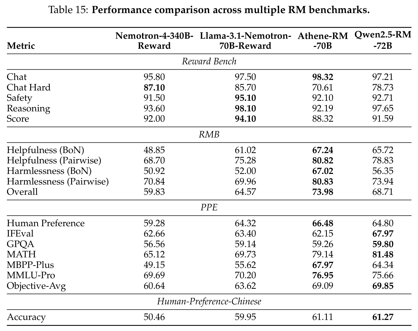
Because the online stage depends on it, the report evaluates Qwen2.5-RM-72B separately. Table 15 compares it with Nemotron-4-340B-Reward, Llama-3.1-Nemotron-70B-Reward and Athene-RM-70B on four benchmarks: Reward Bench, RMB, PPE, and an internal out-of-domain Human-Preference-Chinese set.
No model wins everywhere. Llama-3.1-Nemotron-70B-Reward leads Reward Bench (94.10) and Athene-RM-70B leads RMB (73.98). Qwen2.5-RM-72B leads PPE's objective average (69.85) and Human-Preference-Chinese (61.27), comes second on RMB (68.71), and scores 91.59 on Reward Bench — close to Nemotron-4-340B's 92.00.
The authors draw two conclusions. First, Reward Bench has become the default yardstick, and over-optimising for it looks like Goodhart's law: models that excel there fall back on other benchmarks, which may hurt downstream alignment. Athene-RM-70B scores 88.32 on Reward Bench yet leads RMB. Second, and more important, reward-model benchmark scores did not predict how well the resulting RL policy performed. A higher RM score did not necessarily produce a better RL model. The authors present this as an open research problem, not a solved one.
Key Points
- 1
Benchmarks: Reward Bench, RMB, PPE and an internal Human-Preference-Chinese set
- 2
Reward Bench score: Llama-3.1-Nemotron-70B 94.10, Nemotron-4-340B 92.00, Qwen2.5-RM-72B 91.59, Athene-RM-70B 88.32
- 3
RMB overall: Athene-RM-70B 73.98, Qwen2.5-RM-72B 68.71 (second)
- 4
PPE objective average: Qwen2.5-RM-72B 69.85 (best); Human-Preference-Chinese accuracy: Qwen2.5-RM-72B 61.27 (best)
- 5
Over-optimising for a single RM benchmark can trigger Goodhart's law and degrade performance elsewhere
- 6
Key finding: RM benchmark scores do not reliably predict the quality of the RL model trained with that RM
Pre-training gives Qwen2.5-Turbo the positional range for 1M tokens. Two further problems remain: following instructions over very long inputs, and responding before the user gives up.
For alignment, Turbo's SFT runs in two stages. Stage one uses only short instructions (up to 32,768 tokens) with the same data and steps as the other Qwen2.5 models, which preserves short-task quality. Stage two mixes short instructions with long instructions of up to 262,144 tokens. RL, however, stays short-only. The report gives two reasons: RL on long contexts is computationally expensive, and few reward models can give reliable signals on long inputs. It also reports a useful result: RL on short instructions alone still noticeably improves alignment on long-context tasks.
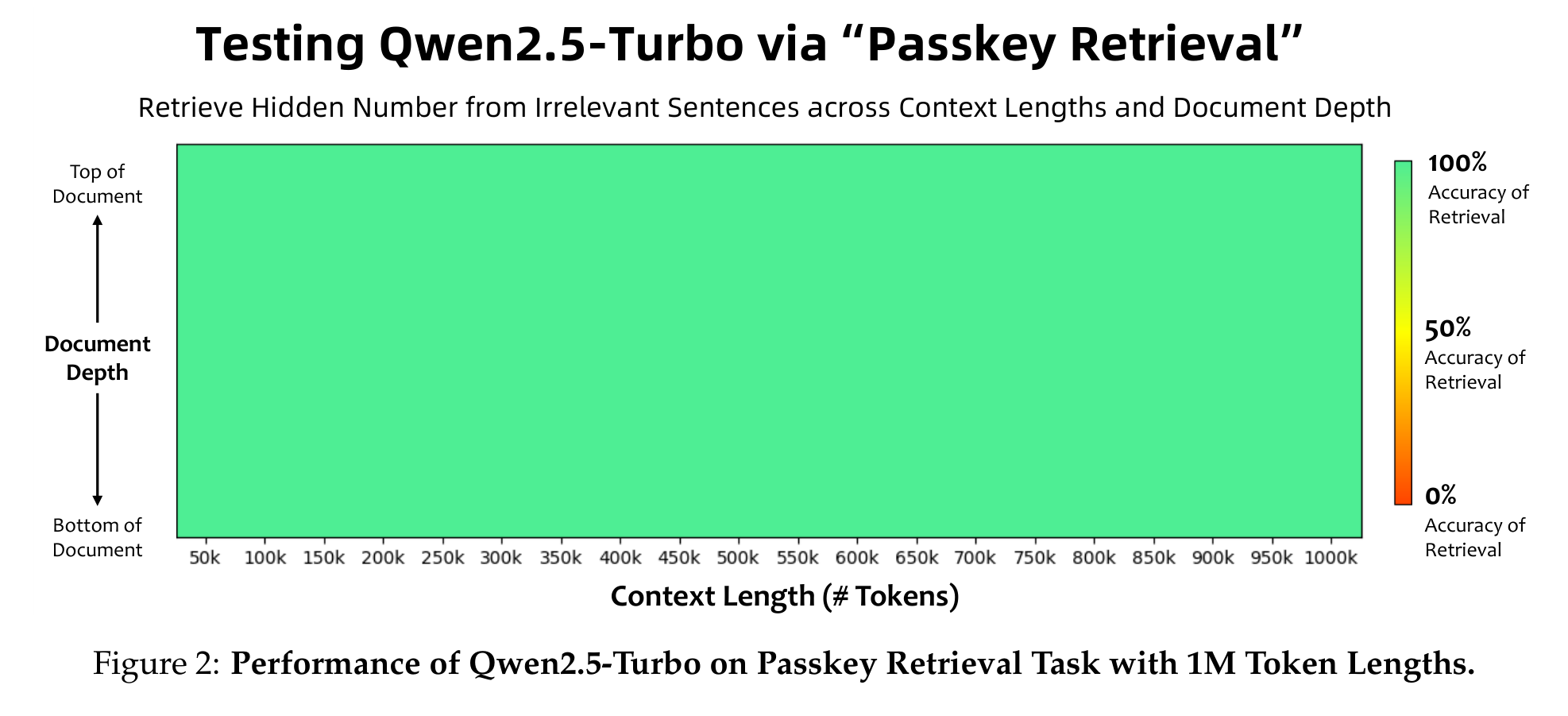
Figure 2 is the retrieval check: Turbo reaches 100% accuracy on 1M-token passkey retrieval at every context length and document depth tested. Figure 3 addresses speed. Full attention over 1M tokens is very slow to prefill, so Qwen2.5 builds a sparse attention mechanism based on MInference that cuts attention computation by 12.5x at 1M tokens. Time to first token falls by 3.2x to 4.3x for Turbo at 1M, depending on hardware (4.3x on H20, 3.2x on A100), and by up to 5.6x for Qwen2.5-7B.
The passkey result should be read in context. Passkey retrieval is the easiest long-context test, since it only requires finding one inserted number. RULER and LV-Eval, covered under Results, are harder tests of whether the model can reason over the whole context.
Key Points
- 1
Turbo SFT stage 1: short instructions only (up to 32,768 tokens), identical to the other Qwen2.5 models
- 2
Turbo SFT stage 2: short + long instructions, long ones up to 262,144 tokens
- 3
RL uses short instructions only — long-context RL is expensive and suitable long-context reward models are scarce — yet still improves long-context alignment
- 4
100% passkey-retrieval accuracy at up to 1M tokens across all document depths (Figure 2)
- 5
Sparse attention based on MInference reduces attention compute by 12.5x at 1M tokens
- 6
Time to first token improves 3.2x–4.3x for Turbo at 1M (A100 / H20), and up to 5.6x for Qwen2.5-7B on H20 (Figure 3)
Mathematical Formulation
Why Prefill Dominates at 1M Tokens
FLOPsattn∝n2d,(3.2×10⁴)2(106)2≈977
Dense attention cost grows quadratically in sequence length n: going from 32K to 1M tokens multiplies attention work by about 1000x. MInference-style sparse attention computes only the query–key blocks that matter, which the report measures as a 12.5x reduction at 1M tokens.
The headline claim is a parameter-efficiency claim: Qwen2.5-72B-Instruct is competitive with Llama-3.1-405B-Instruct, a model about 5.6x larger. The abstract says "around 5 times larger" and the conclusion says "six times smaller"; the actual ratio 405/72≈5.6 falls between them.
Base models (Table 2). Qwen2.5-72B scores 86.1 MMLU, 62.1 MATH, 91.5 GSM8K and 84.7 MBPP, against Llama-3-405B's 85.2, 53.8, 89.0 and 73.0. It is not better on every row: on HumanEval it scores 59.1, below Qwen2-72B (64.6) and Llama-3-405B (61.0). Qwen2.5-Plus reaches 64.0 MMLU-Pro, 5.9 points above Qwen2.5-72B.
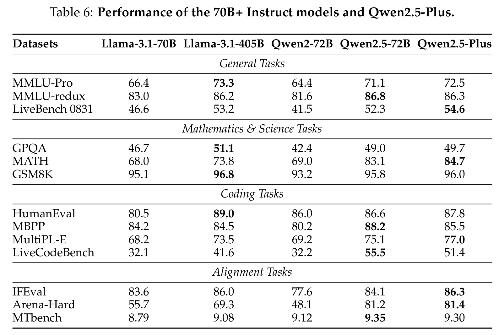
Instruction-tuned models (Table 6). Qwen2.5-72B-Instruct beats Llama-3.1-405B-Instruct on MMLU-redux (86.8 vs 86.2), MATH (83.1 vs 73.8), MBPP (88.2 vs 84.5), MultiPL-E (75.1 vs 73.5), LiveCodeBench (55.5 vs 41.6), Arena-Hard (81.2 vs 69.3) and MT-Bench (9.35 vs 9.08). It trails on the other six: MMLU-Pro (71.1 vs 73.3), LiveBench (52.3 vs 53.2), GPQA (49.0 vs 51.1), GSM8K (95.8 vs 96.8), HumanEval (86.6 vs 89.0) and IFEval (84.1 vs 86.0). Qwen2.5-Plus beats Qwen2.5-72B-Instruct on 9 of 13 benchmarks, which matches the table.
Smaller models. Qwen2.5-7B-Instruct scores 75.5 on MATH and 84.8 on HumanEval, against Gemma2-9B's 44.3 and 68.9. Qwen2.5-3B-Instruct reaches 65.9 MATH with 2.8B non-embedding parameters. One claim does not match its table: the report says Qwen2.5-Turbo beats Qwen2.5-14B-Instruct on "eight out of ten benchmarks," but Table 7 has 13 rows and Turbo leads on 6 of them (MMLU-Pro, MMLU-redux, MATH, HumanEval, MBPP, MultiPL-E).
Long context (Table 16). Qwen2.5-72B-Instruct averages 95.1 on RULER and scores 88.4 at 128K, ahead of GPT-4 (81.2) and Llama-3.1-70B (66.6). The ablation rows isolate YaRN + DCA: without them, 72B falls to 67.0 at 128K and 7B to 31.4 (from 55.1). On LV-Eval at 256K, 72B scores 45.2 with the extension methods and 2.4 without.
All evaluations use the same decontamination rule as Qwen2: a training sequence is removed if its longest common subsequence with any test sequence is at least 13 tokens and covers at least 60% of the shorter sequence.
Key Points
- 1
Qwen2.5-72B-Instruct vs Llama-3.1-405B-Instruct: wins on MMLU-redux, MATH (83.1 vs 73.8), MBPP, MultiPL-E, LiveCodeBench (55.5 vs 41.6), Arena-Hard (81.2 vs 69.3) and MT-Bench — 7 of 13; trails on MMLU-Pro, LiveBench, GPQA, GSM8K, HumanEval and IFEval
- 2
Base Qwen2.5-72B: 86.1 MMLU, 62.1 MATH, 91.5 GSM8K, 84.7 MBPP — but HumanEval drops to 59.1 from Qwen2-72B's 64.6
- 3
Qwen2.5-Plus beats Qwen2.5-72B-Instruct on 9 of 13 instruct benchmarks and reaches 64.0 base MMLU-Pro
- 4
Qwen2.5-7B-Instruct: 75.5 MATH, 84.8 HumanEval; Qwen2.5-3B-Instruct: 65.9 MATH with 2.8B non-embedding parameters
- 5
Paper vs table: the "Turbo beats 14B-Instruct on eight of ten" claim does not match Table 7 (Turbo leads on 6 of 13 rows)
- 6
RULER at 128K: 72B-Instruct 88.4 with YaRN + DCA vs 67.0 without; GPT-4 scores 81.2
- 7
Size ratio: 405/72≈5.6 — the paper says "around 5 times" in the abstract and "six times" in the conclusion
Mathematical Formulation
Decontamination Rule
remove st⟺∃se:∣LCS(st,se)∣≥13∧∣LCS(st,se)∣≥0.6×min(∣st∣,∣se∣)
A training sequence st is removed if it shares a longest common subsequence with some test sequence se that is both at least 13 tokens long and at least 60% of the shorter of the two. The rule is applied to both pre-training and post-training data.
Keep reading
Related Papers
Go deeper